| Franz J. Vesely > CompPhys Tutorial > Partial Differential Equations |
INDEX
INDEX
Start/Contents
Start/Contents
Preamble
Preamble
1 FINITE DIFFERENCES
1 FINITE DIFFERENCES
Definitions
Definitions
Interpolation Formulae
Interpolation Formulae
Differential Quotients
Differential Quotients
Differencing in 2D
Differencing in 2D
Sample Applications
Sample Applications
2 LINEAR ALGEBRA
2 LINEAR ALGEBRA
Exact Methods
Exact Methods
Relaxation Methods
Relaxation Methods
Conjugate Gradients
Conjugate Gradients
Eigenvalues and -vectors
Eigenvalues and -vectors
Sample Applications
Sample Applications
3 STOCHASTICS
3 STOCHASTICS
Equidistributed random variates
Equidistributed random variates
Other Distributions
Other Distributions
Random Processes
Random Processes
Stochastic Optimization
Stochastic Optimization
4 ORDINARY DE
4 ORDINARY DE
Definitions
Definitions
IVP First Order
IVP First Order
IVP Second Order
IVP Second Order
BVP
BVP
5 PARTIAL DE
5 PARTIAL DE
IVP I: Hyperbolic
IVP I: Hyperbolic
IVP II: Parabolic
IVP II: Parabolic
BVP: Elliptic
BVP: Elliptic
6 SIMULATION
6 SIMULATION
Model Systems
Model Systems
Monte Carlo
Monte Carlo
Molecular Dynamics
Molecular Dynamics
Evaluation of Simulations
Evaluation of Simulations
Long ranged Potentials
Long ranged Potentials
Stochastic Dynamics
Stochastic Dynamics
7 QUANTUM M.
7 QUANTUM M.
Diffusion MC
Diffusion MC
Path Integral MC
Path Integral MC
Wave Packet Dynamics
Wave Packet Dynamics
Density Functional MD
Density Functional MD
8 HYDRODYN.
8 HYDRODYN.
Compressible, no Viscosity
Compressible, no Viscosity
Incompressible, with Viscosity
Incompressible, with Viscosity
Lattice Gas Models
Lattice Gas Models
Bird's Direct Simulation MC
Bird's Direct Simulation MC
APPENDICES
APPENDICES
Machine Errors
Machine Errors
Discrete Fourier Transformation
Discrete Fourier Transformation
Exercises and Projects
Exercises and Projects
Some Good Books
Some Good Books
Bibliography
Bibliography
5.2 Initial Value Problems II: Conservative-parabolic DEDiffusion: tu=x( tu=x( xu)ortu=x22u xu)ortu=x22uBest: 2 second-order schemes - Crank-Nicholson - Dufort-Frankel But: first-order algorithms perform well, too - FTCS (one up for old Leonhard E.!) - Implicit (even better - good enough for many purposes!) Subsections
5.2.1 FTCS Scheme for Parabolic DEInu t=2ux2ut2ux2 t=2ux2ut2ux2  t t ujn+1–ujn ujn+1–ujn = (x)2unj+1–2ujn+unj–1 = (x)2unj+1–2ujn+unj–1 Using  t(x)2 t(x)2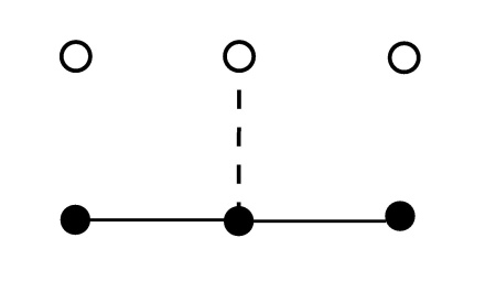
For the
\Delta t \leq \frac{\textstyle (\Delta x)^{2}}{\textstyle 2\lambda} \equiv \tau
where \tau is the characteristic time for the diffusion over a distance \Delta x (i.e. one lattice space). The FTCS scheme is simple and stable, but inefficient. EXERCISE: Remember the thermal conduction problem we considered earlier? If you haven't done it then, do it now, using FTCS. Interpret the behavior of the solution for varying time step sizes in the light of the above stability considerations. 5.2.2 Implicit Scheme of First OrderTake the second spatial derivative at time t_{n+1} instead of t_{n}:
\frac{\textstyle 1}{\textstyle \Delta t}
\left[ u_{j}^{n+1}-u_{j}^{n}\right]
= \frac{\textstyle \lambda}{\textstyle (\Delta x)^{2}}
\left[ u_{j+1}^{n+1}-2 u_{j}^{n+1}+u_{j-1}^{n+1}\right]
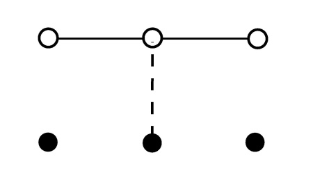
Again defining a \equiv \lambda \Delta t / (\Delta x)^{2}, we find, for each space point x_{j} \;(j=1,2,..N-1),
-a u_{j-1}^{n+1}+(1+2a)u_{j}^{n+1}-a u_{j+1}^{n+1}=u_{j}^{n}
Let the boundary values u_{0} and u_{N} be given; the set of equations may then be written as
A \cdot u^{n+1} = u^{n}
with
\begin{eqnarray}
A & \equiv &
\left(
\begin{array}{cccccc}
1 & 0 & 0 & . & . & 0 \\
-a & 1+2a & -a & 0 & . & 0 \\
0 & . & . & . & 0 & . \\
. & . & . & . & . & . \\
. & . & . & -a & 1+2a & -a \\
. & . & . & 0 & 0 & 1
\end{array}
\right)
\end{eqnarray}
\Longrightarrow Solve by Recursion! Stability: We find
g = \frac{\textstyle 1}{\textstyle 1+4a\sin^{2}(k \Delta x/2)}
Since \vert g\vert \leq 1 under all circumstances, we have here an unconditionally stable algorithm! EXERCISE: Apply the implicit technique to the thermal conduction problem discussed before. Consider the efficiency of the procedure as compared to FTCS. Relate the problem to the Wiener-Levy random walk. 5.2.3 Crank-Nicholson Scheme (CN)As before, replace \partial u/ \partial t by \Delta_{n} u/\Delta t \equiv (u^{n+1}-u^{n})/\Delta t.Noting that this approximation is in fact centered at t_{n+1/2}, introduce the same kind of time centering on the right-hand side: taking the mean of \delta_{j}^{2}u^{n} (= FTCS) and \delta_{j}^{2}u^{n+1} (= implicit scheme) we write
\frac{\textstyle 1}{\textstyle \Delta t}
\left[ u_{j}^{n+1}-u_{j}^{n} \right]
= \frac{\textstyle \lambda}{\textstyle 2(\Delta x)^{2}}
\left[ (u_{j+1}^{n+1}-2 u_{j}^{n+1}+u_{j-1}^{n+1})
+ (u_{j+1}^{n}-2 u_{j}^{n}+u_{j-1}^{n}) \right]
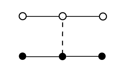
The Crank-Nicholson formula is of second order in \Delta t. Defining a \equiv \lambda \Delta t / 2(\Delta x)^{2} we may write CN as
-a u_{j-1}^{n+1}+(1+2a)u_{j}^{n+1}-a u_{j+1}^{n+1}=
a u_{j-1}^{n}+(1-2a)u_{j}^{n}+a u_{j+1}^{n}
or
A \cdot u^{n+1} = B \cdot u^{n}
with
A \! \equiv \!
\left(
\begin{array}{cccccc}
1 & 0 & 0 & . & . & 0 \\
-a & 1\!+\!2a & -a & 0 & . & 0 \\
0 & . & . & . & 0 & . \\
. & . & . & . & . & . \\
. & . & . & -a & 1\!+\!2a & -a \\
. & . & . & 0 & 0 & 1
\end{array}
\right) \;\;
B \! \equiv \!
\left(
\begin{array}{cccccc}
1 & 0 & 0 & . & . & 0 \\
a & 1\!-\!2a & a & 0 & . & 0 \\
0 & . & . & . & 0 & . \\
. & . & . & . & . & . \\
. & . & . & a & 1\!-\!2a & a \\
. & . & . & 0 & 0 & 1
\end{array}
\right)
Tridiagonal \Longrightarrow Solve by Recursion! Stability of CN: The amplification factor is
g(k)=\frac{\textstyle 1-2a\sin^{2}(k\Delta x/2)}{\textstyle 1+2a\sin^{2}(k\Delta x/2)}
\leq 1 \; ,
which makes the CN method unconditionally stable. EXAMPLE: The time-dependent Schroedinger equation,
\frac{\textstyle \partial u}{\textstyle \partial t}
= -i H u \; , \;\;\; {\rm with} \;\; H \equiv
\frac{\textstyle \partial^{2}}{\textstyle \partial x^{2}} + U(x)
when rewritten à la Crank-Nicholson, reads
\frac{\textstyle 1}{\textstyle \Delta t}[u_{j}^{n+1}-u_{j}^{n}]
= - \frac{\textstyle i}{\textstyle 2} [(Hu)_{j}^{n+1}+(Hu)_{j}^{n}]
= - \frac{\textstyle i}{\textstyle 2}
\left[ \frac{\textstyle \delta_{j}^{2}u_{j}^{n+1}}{\textstyle (\Delta x)^{2}}
+U_{j}u_{j}^{n+1}
+\frac{\textstyle \delta_{j}^{2}u_{j}^{n}}{\textstyle (\Delta x)^{2}}
+U_{j}u_{j}^{n} \right]
With a \equiv \Delta t/2 (\Delta x)^{2} and b_{j} \equiv U(x_{j}) \Delta t/2 this leads to
\begin{eqnarray}
(ia) u_{j-1}^{n+1}+(1-2ia+ib_{j})u_{j}^{n+1}&\!+&\!(ia) u_{j+1}^{n+1}=
\\
&&
=(-ia) u_{j-1}^{n}+(1+2ia-ib_{j})u_{j}^{n}+(-ia) u_{j+1}^{n}
\end{eqnarray}
Again, we have a tridiagonal system which may be inverted very efficiently by recursion. 5.2.4 Dufort-Frankel Scheme (DF)DST in time and space, but in place of -2u_{j}^{n} use -(u_{j}^{n+1}+u_{j}^{n-1}):
\frac{\textstyle 1}{\textstyle 2 \Delta t} \left[ u_{j}^{n+1}-u_{j}^{n-1} \right]
= \frac{\textstyle \lambda}{\textstyle (\Delta x)^{2}}
\left[ u_{j+1}^{n}-(u_{j}^{n+1}+u_{j}^{n-1})+u_{j-1}^{n} \right]
or, with a \equiv 2 \lambda \Delta t/(\Delta x)^{2},
\begin{eqnarray}
&&
u_{j}^{n+1} = \frac{\textstyle 1-a}{\textstyle 1+a}u_{j}^{n-1}
+ \frac{\textstyle a}{\textstyle 1+a}
\left[ u_{j+1}^{n}+ u_{j-1}^{n}\right]
\end{eqnarray}
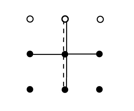
The DF algorithm is of second order in \Delta t. In contrast to CN, it is an explicit expression for u_{j}^{n+1}. Stability:
g =\frac{\textstyle 1}{\textstyle 1+a} \left[ a \cos k \Delta x \pm
\sqrt{1-a^{2}\sin^{2}k \Delta x} \right]
Considering in turn the cases a^{2}\sin^{2}k \Delta x \geq 1 and \dots < 1 we find that |g|^{2} \leq 1 always; the method is unconditionally stable. 5.2.5 Resumé: Conservative-parabolic DE
\frac{\textstyle \partial u}{\textstyle \partial t}
= \lambda \frac{\textstyle \partial^{2} u}{\textstyle \partial x^{2}}
- Use Crank-Nicholson! (2nd order implicit scheme; needs recursion) - If too lazy for implicit scheme, use Dufort-Frankel (2nd order explicit) - If 1st order is sufficient, use implicit scheme vesely 2006-01-23
|