| Franz J. Vesely > CompPhys Tutorial > Differential Equations |
4.1 Initial Value Problems of First Order2 guinea pigs will often be used:(1) Relaxation equation
$
\begin{eqnarray}
\frac{\textstyle dy}{\textstyle dt}&=&-\lambda y , \;\;\; {\rm with} \;\;
y(t=0)=y_{0}
\end{eqnarray}
$
(2) Harmonic oscillator in linear form
$
\begin{eqnarray}
\frac{\textstyle dy}{\textstyle dt}& = & L \cdot y,\;\;\;\;{\rm where}\;\;
y \equiv \left(\begin{array}{r} x \\ \\v \end{array} \right) \;\;\; {\rm and}\;\;
L = \left( \begin{array}{cc}0&1\\ \\-\omega_{0}^{2} & 0 \end{array} \right)
\end{eqnarray}
$
Subsections:
4.1.1 Euler-Cauchy AlgorithmApply DNGF approximation
$
\begin{eqnarray}
\left. \frac{\textstyle d y}{\textstyle dt} \right|_{t_{n}} & = &
\frac{\textstyle \Delta y_{n}}{\textstyle \Delta t} + O[(\Delta t)]
\end{eqnarray}
$
to the linear DE and find the Euler-Cauchy (EC) formula
$
\begin{eqnarray}
\frac{\textstyle \Delta y_{n}}{\textstyle \Delta t} & = & f_{n} + O[(\Delta t)]
\end{eqnarray}
$
or
$
y_{n+1}= y_{n}+ f_{n} \Delta t + O[(\Delta t)^{2}]
$
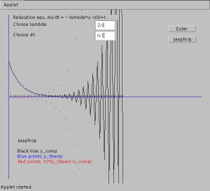
Algebraically and computationally simple, but useless: - Only first order accuracy - Unstable: small aberrations from the true solution tend to grow in the course of further steps: Demo: Apply EC to the relaxation equation $\frac{\textstyle dy(t)}{\textstyle dt}=-\lambda y(t)$:
$
\begin{eqnarray}
y_{n+1} & = & (1-\lambda \Delta t) y_{n}
\end{eqnarray}
$
EC applied to the equation $dy/dt=-\lambda y$, with $\lambda =1$ and $y_{0}=1$: unstable for $\lambda \Delta t > 2$ Therefore: some considerations on the accuracy and stability of such schemes are necessary. 4.1.2 Stability and Accuracy of Difference SchemesLet $ y(t)$ be the exact solution of a DE, and $ e(t)$ an error: at time $t_{n}$, the algorithm produces $ y_{n}+ e_{n}$.$\Longrightarrow$ $t_{n+1}$? For EC, $ y_{n+1}+ e_{n+1}= y_{n}+ e_{n}+ f( y_{n}+ e_{n}) \Delta t$. Generally,
$
\begin{eqnarray}
y_{n+1}+ e_{n+1} & = & T( y_{n}+ e_{n})
\end{eqnarray}
$
Expand around the correct solution:
$
\begin{eqnarray}
T( y_{n}+ e_{n}) & \approx & T( y_{n})+
\left. \frac{\textstyle dT(y)}{\textstyle dy} \right|_{y_{n}} \cdot e_{n}
\end{eqnarray}
$
or
$
\begin{eqnarray}
e_{n+1} & \approx &
\left. \frac{\textstyle dT( y)}{\textstyle d y} \right|_{ y_{n}} \cdot e_{n}
\equiv G \cdot e_{n}
\end{eqnarray}
$
The matrix $G$ is called amplification matrix. All its eigenvalues must be within the unit circle:
$
\begin{eqnarray}
|g_{i}| &\leq& 1 ,\;\; {\rm for \; all\; \it i}
\end{eqnarray}
$
EXAMPLE: EC + Relaxation equation
$
\begin{eqnarray}
T(y_{n}) & \equiv & (1-\lambda \Delta t) y_{n}
\end{eqnarray}
$
$\Longrightarrow$
$
\begin{eqnarray}
|1-\lambda \Delta t| & \leq & 1
\end{eqnarray}
$
For $\lambda =1$ this condition is met whenever $\Delta t \leq 2$. $\Longrightarrow$ Check the previous figure! EXAMPLE: EC + Harmonic oscillator
$
\begin{eqnarray}
y_{n+1} & = &[I+ L \Delta t] \cdot y_{n} \equiv T( y_{n})
\end{eqnarray}
$
The amplification matrix is
$
\begin{eqnarray}
G & \equiv & \left. \frac{\textstyle dT(y)}{\textstyle d y} \right|_{ y_{n}} =
I+ L \Delta t
\end{eqnarray}
$
with eigenvalues $g_{1,2}=1 \pm i \omega_{0} \Delta t$, so that
$
\begin{eqnarray}
|g_{1,2}| & = & \sqrt{1+(\omega_{0} \Delta t)^{2}} > 1 \;\;\;{\rm always!!}
\end{eqnarray}
$
$\Longrightarrow$ EC applied to the harmonic oscillator is never stable.
4.1.3 Explicit Methods- Euler-Cauchy (from DNGF; see above)- Leapfrog algorithm (from DST):
$
\begin{eqnarray}
y_{n+1}&=& y_{n-1}+ f_{n} 2\Delta t
+ O[(\Delta t)^{3}] \\
y_{n+2}&=& y_{n}+ f_{n+1} 2\Delta t + O[(\Delta t)^{3}]
\end{eqnarray}
$
This is an example of a multistep technique, as timesteps $t_{n}$ and $t_{n-1}$ contribute to $y(t_{n+1})$. Stability analysis for such algorithms is as follows: Let the explicit multistep scheme be written as
$
y_{n+1}=\sum \limits_{j=0}^{k}
\left[ a_{j} y_{n-j}+b_{j}\Delta t f_{n-j} \right]
$
Inserting a slightly deviating solution $ y_{n-j}+ e_{n-j}$ and computing the difference, we have
$
e_{n+1} \approx \sum \limits_{j=0}^{k} \left[ a_{j} I+b_{j} \Delta t
\left. \frac{\textstyle df}{\textstyle d y} \right|_{ y_{n-j}} \right] \cdot
e_{n-j} \equiv \sum \limits_{j=0}^{k} A_{j} \cdot e_{n-j}
$
We combine the errors at subsequent time steps to a vector
$
\eta_{n} \equiv \left(
\begin{array}{l}
e_{n} \\ e_{n-1} \\ \vdots \\ e_{n-k}
\end{array} \right)
$
and define the quadratic matrix
$
G \equiv
\left(
\begin{array}{cccc}
A_{0} & A_{1} & \dots & A_{k} \\
I & 0 & \dots & 0 \\
0 & \ddots & & 0 \\
0 & \dots & I & 0 \\
\end{array}
\right)
$
Then
$
\eta_{n+1}= G \cdot \eta_{n}
$
Stability is guaranteed if
$
|g_{i}| \leq 1 ,\;\; {\rm for\; all \; \it i}
$
EXAMPLE 1: Leapfrog / Relaxation equation:
$
y_{n+1} = y_{n-1}-2 \Delta t \lambda y_{n} +O[(\Delta t)^{3}]
$
Therefore
$
e_{n+1} \approx -2\Delta t \lambda e_{n} + e_{n-1}
$
which means that $A_{0} = -2 \Delta t \lambda$, and $A_{1}=1$, and the matrix $G$ is
$
G = \left( \begin{array}{cc}-2\Delta t \lambda & 1 \\ \\1 & 0 \end{array} \right)
$
with eigenvalues
$
g_{1,2} = -\lambda \Delta t \pm \sqrt{(\lambda \Delta t)^{2}+1}
$
For real $\lambda \Delta t$ we find that $\vert g_{2}\vert > 1$ always, meaning that the leapfrog scheme is unstable for the relaxation (or growth) equation.
EXAMPLE 2: Leapfrog / Harmonic oscillator:
$ y_{n+1}=2\Delta t { L} \cdot y_{n} + y_{n-1}$
and
$ e_{n+1} \approx 2\Delta t { L} \cdot e_{n} + e_{n-1}$
For the amplification matrix we find (with $\alpha \equiv 2 \Delta t$)
$
G = \left(\begin{array}{cc}\alpha L & I \\ \\ I & 0 \end{array} \right) =
\left(
\begin{array}{cccc}
0 & \alpha & 1 & 0 \\
-\alpha \omega_{0}^{2} & 0 & 0 & 1 \\
1 & 0 & 0 & 0 \\
0 & 1 & 0 & 0
\end{array}
\right)
$
with eigenvalues
$
g= \pm \left[ (1-\frac{\textstyle \alpha^{2} \omega_{0}^{2}}{\textstyle 2})
\pm i \alpha \omega_{0}
\sqrt{1-\frac{\textstyle \alpha^{2} \omega_{0}^{2}}{\textstyle 4}} \; \right]^{1/2}
$
But the modulus of this is always $\vert g \vert=1$. $\Longrightarrow$ The leapfrog algorithm is marginally stable for the harmonic oscillator. 4.1.4 Implicit MethodsMuch more stable!- First order scheme (from DNGB): Insert
$
\begin{eqnarray}
\left. \frac{\textstyle dy}{\textstyle dt} \right|_{n+1} & = &
\frac{\textstyle \nabla y_{n+1}}{\textstyle \Delta t}+O[\Delta t]
\end{eqnarray}
$
in $dy/dt=f[y(t)]$ to find
$
\begin{eqnarray}
y_{n+1} & = & y_{n}+ f_{n+1} \Delta t + O[(\Delta t)^{2}]
\end{eqnarray}
$
If $ f(y)$ is linear, $ f_{n+1}= L \cdot y_{n+1}$:
$
y_{n+1} = [ I- L \Delta t]^{-1} \cdot y_{n} + O[(\Delta t)^{2}]
$
Stability:
$
e_{n+1} = [I - L \Delta t]^{-1} \cdot e_{n}
\equiv { G} \cdot e_{n}
$
EXAMPLES: (a) Relaxation equation: $ G = 1/(1+\lambda \Delta t)$, thus $\vert g\vert<1$ for any $\lambda>0$. (b) Harmonic oscillator:
$
G \equiv [I- L \Delta t]^{-1} =
\frac{\textstyle 1}{\textstyle 1+(\omega_{0} \Delta t)^{2}}
\left(\begin{array}{cc}1&\Delta t\\ \\ -\omega_{0}^{2}\Delta t & 1\end{array} \right)
$
with eigenvalues
$
g_{1,2}=\frac{\textstyle 1}{\textstyle 1+(\omega_{0} \Delta t)^{2}}
[1 \pm i \omega_{0} \Delta t]
$
Thus
$
|g|^{2}=\frac{\textstyle 1}{\textstyle 1+(\omega_{0} \Delta t)^{2}} < 1 \;\;\;
{\rm for}\;\;{\rm all}\;\; \Delta t
$
$\Longrightarrow$ Method is always stable for relaxation equation and harmonic oscillator. - Second order implicit scheme (from adding the DNGF formulae at $t_{n}$ and $t_{n+1}$, respectively):
$
\begin{eqnarray}
y_{n+1} & = & y_{n} +\frac{\textstyle \Delta t}{\textstyle 2}[ f_{n}+ f_{n+1}]
+O[(\Delta t)^{3}]
\end{eqnarray}
$
If $ f_{n}= L \cdot y_{n}$ etc.:
$
\begin{eqnarray}
y_{n+1}=[I-L \frac{\textstyle \Delta t}{\textstyle 2}]^{-1} \cdot
[I+L \frac{\textstyle \Delta t}{\textstyle 2}] \cdot y_{n}
+O[(\Delta t)^{3}]
\end{eqnarray}
$
Always stable for relaxation equation and harmonic oscillator. 4.1.5 Predictor-Corrector Method
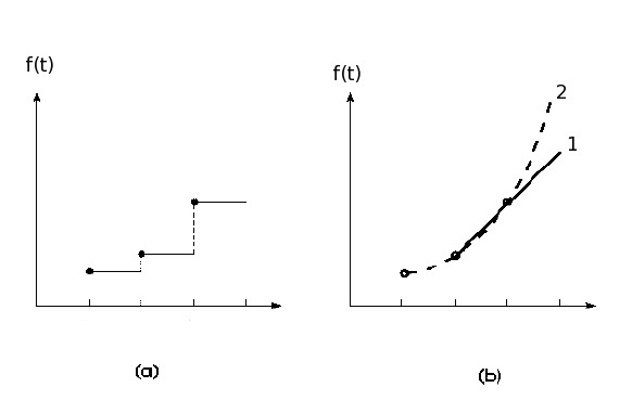
Predictor step: - Extrapolate the function $f(t)$, using an NGB polynomial, into $[t_{n}, t_{n+1}]$. - Formally integrate the r.h.s. in $dy/dt=f(t)$ to arrive at the Adams-Bashforth predictor:
$
\begin{eqnarray}
y^{P}_{n+1} & = & y_{n}+\Delta t \left[ f_{n} + \frac{1}{2} \nabla f_{n}
+ \frac{5}{12} \nabla^{2} f_{n}+ \frac{3}{8} \nabla^{3} f_{n} +
\dots \right]
\end{eqnarray}
$
- Truncate at some term to obtain the various predictors in the table.
Predictors for first order differential equations:
$ \begin{eqnarray} y^{P}_{n+1}=y_{n} &+& \Delta t f_{n} + O[(\Delta t)^{2}] \;\;\;\;{\rm (Euler-Cauchy!)} \\ \dots &+& \frac{\textstyle \Delta t}{\textstyle 2}[3 f_{n}-f_{n-1}] + O[(\Delta t)^{3}] \\ \dots &+& \frac{\textstyle \Delta t}{\textstyle 12}[23 f_{n}-16f_{n-1} + 5f_{n-2}] + O[(\Delta t)^{4}] \\ \dots &+& \frac{\textstyle \Delta t}{\textstyle 24}[55 f_{n}-59f_{n-1} + 37f_{n-2} - 9f_{n-3}] + O[(\Delta t)^{5}] \\ \vdots && \end{eqnarray} $ Adams-Bashforth predictors Evaluation step: As soon as the predictor $y^{P}_{n+1}$ is available, insert it in $f(y)$:
$
\begin{eqnarray}
f_{n+1}^{P} &\equiv& f[y_{n+1}^{P}]
\end{eqnarray}
$
Corrector step: - Again back-interpolate the function $f(t)$, using NGB, but now starting at $t_{n+1}$. - Formally re-integrate the r.h.s. in $dy/dt=f(t)$ to find the Adams-Moulton corrector:
$
\begin{eqnarray}
y_{n+1}&=&y_{n}+\Delta t \left[ f_{n+1} - \frac{1}{2} \nabla f_{n+1}
- \frac{1}{12} \nabla^{2} f_{n+1} - \frac{1}{24} \nabla^{3} f_{n+1}
- \dots \right]
\end{eqnarray}
$
Correctors for first order differential equations:
$ \begin{eqnarray} y_{n+1}=y_{n} &+& \Delta t f_{n+1}^{P} + O[(\Delta t)^{2}] \\ \dots &+& \frac{\textstyle \Delta t}{\textstyle 2} [f_{n+1}^{P}+f_{n}] + O[(\Delta t)^{3}] \\ \dots &+& \frac{\textstyle \Delta t}{\textstyle 12} [5 f_{n+1}^{P}+8f_{n} - f_{n-1}] + O[(\Delta t)^{4}] \\ \dots &+& \frac{\textstyle \Delta t}{\textstyle 24} [9 f_{n+1}^{P}+19f_{n} - 5f_{n-1} + f_{n-2}] + O[(\Delta t)^{5}] \\ \vdots && \end{eqnarray} $ Adams-Moulton correctors Finally: evaluate $f_{n+1} \equiv f(y_{n+1})$. Stability of PC schemes: Intermediate between the lousy explicit and the excellent implicit methods. EXAMPLE: 2nd order PC + relaxation equation: stable for $\Delta t \leq 2/\lambda$. (The bare predictor would have $\Delta t \leq 1/\lambda$.) 4.1.6 Runge-Kutta Method
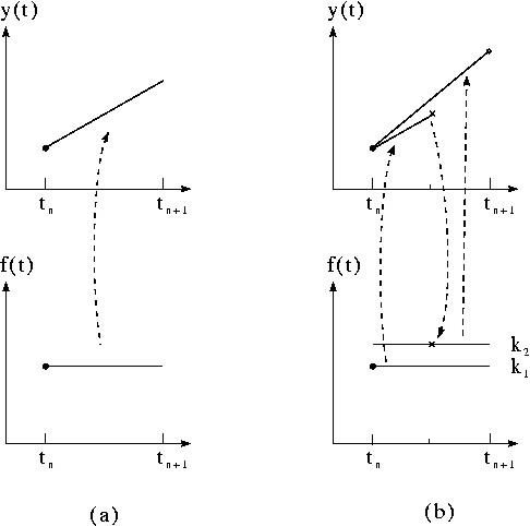
Runge-Kutta of order 2:
$ \begin{eqnarray} k_{1} & = & \Delta t \, f(y_{n}) \\ k_{2} & = & \Delta t \, f(y_{n} + \frac{1}{2}k_{1}) \\ y_{n+1} & = & y_{n}+k_{2}+O[(\Delta t)^{3}] \end{eqnarray} $ (Also called half-step method, or Euler-Richardson algorithm.) A much more powerful method that has found wide application is the RK algorithm of order 4, as described in the table.
Runge-Kutta of order 4 for first-order ODE:
Advantages of RK: - Self-starting (no preceding $y_{n-1} \dots$ needed) - Adjustable $\Delta t$
But:
Stability of RK: vesely 2005-10-10
|