The structure of recent philosophy (II)
Contents
An older version of my philosophy-maps . I’m mainly keeping it around, because it contains some useful code.
In this codebook we will investigate the macro-structure of philosophical literat ure. As a base for our investigation I have collected about fifty-thousand records from the Web of Science collection, spanning from the late forties to this very day.
The question of how philosophy is structured has received quite a lot of attention, albeit usually under more specific formulations, for example when people ask whether there is a divide between “analytic” and “continental” philosophy, or whether philosophy is divided more along the lines of “naturalism” and “anti-naturalism”. I think that the toolkit I provide below allows to give answers to these questions. As it is purely data-driven, it is free from most prior assumptions about how philosophy is structured. And because it encompasses a rather large sample of philosophical literature, it should guide us to a point of view, that is cleared from the personal expectations that we have from our own intellectual histories.
We will focus in this post mostly on the visualization aspect, to build some intuitions about the structure of the philosophical literature and will not attempt to answer specific questions.
This work makes use of several great python libraries. I would like to note specifically:
- Metaknowledge which we will use to parse the data from the WebOfScience-data.
- UMAP which we will use for the embedding of the data.
- hdbscan which we will use to do the clustering.
Note: This is the second online version of this project. It differs from the first in the following aspects:
- It uses a different, and I think more advanced method of vectorization.
- I have fixed an error in the data spotted by Fabio Votta.
- I updated the visualization technique.
- I cluster on the 2-dimensional umap, not on the thirty dimensional, which works surprisingly well.
Literature
McInnes L, Healy J. Accelerated Hierarchical Density Based Clustering In: 2017 IEEE International Conference on Data Mining Workshops (ICDMW), IEEE, pp 33-42. 2017
McInnes, L, Healy, J, UMAP: Uniform Manifold Approximation and Projection for Dimension Reduction, ArXiv e-prints 1802.03426, 2018
Reid McIlroy-Young, John McLevey, and Jillian Anderson. 2015. metaknowledge: open source software for social networks, bibliometrics, and sociology of knowledge research. URL: http://www.networkslab.org/metaknowledge.
 1
 2
 3
 4
 5
 6
 7
 8
 9
10
11
12
13
14
15
16
17
18
19
import metaknowledge as mk import pandas as pd import numpy as np from random import randint import datetime import scipy as scipy %matplotlib inline import seaborn as sns import matplotlib.pyplot as plt #For Tables: from IPython.display import display from IPython.display import Latex pd.set_option('display.max_columns', 500) #For R (ggplot2) %load_ext rpy2.ipythonThe rpy2.ipython extension is already loaded. To reload it, use: %reload_ext rpy2.ipython
The WOS-Files where collected with a threefold snowball-sampling strategy. I started out with eight pretty different journals:
- Analysis
- The Papers of the British Society for Phenomenology
- The Continental Philosophy Review
- Erkenntnis
- Ethics
- The Journal of speculative Philosophy
- Mind
- Philosophical Quarterly
- Philosophy and Social Criticism
These should provide a pretty diverse entry-point into philosophy. Of each journal I collected the 500 most cited papers, and analysed, which journals these papers cited. Of those journals I evaluated the citations of the top 500 papers of the 30 most cited journals (a total of around 15000 papers). Thus I arrived at a list of fifty philosophy journals, that should, by every sensible criterion, be a good aproximation for whatever philosophers have been interested in. I downloaded for each of this journals every record in the WOS-Database, arriving at collection of 56062 records.
Now, without further ado, lets load our raw data, filter out incomplete records and print a little summary of it.
|
|
|
|
RecordCollection glimpse made at: 2018-09-16 00:13:50
53491 Records from Empty

Top Authors
1 SHELAH, S
2 Shelah, S
2 HINTIKKA, J
3 MARGOLIS, J
4 LOWE, EJ
5 LEWIS, D
6 SOBER, E
7 KITCHER, P
8 RESCHER, N
9 CHISHOLM, RM
9 PARGETTER, R
10 Nanay, Bence
10 JACKSON, F
10 Turri, John
10 CASTANEDA, HN
11 Douven, Igor
12 PETTIT, P
13 Brueckner, A
13 Brogaard, Berit
13 SORENSEN, RA
14 Carter, J. Adam
14 VANFRAASSEN, BC

Top Journals
1 SYNTHESE
2 PHILOSOPHICAL STUDIES
3 JOURNAL OF SYMBOLIC LOGIC
4 PHILOSOPHY OF SCIENCE
5 PHILOSOPHY AND PHENOMENOLOGICAL RESEARCH
6 ANALYSIS
7 JOURNAL OF PHILOSOPHY
8 MONIST
9 PHILOSOPHY
10 SOUTHERN JOURNAL OF PHILOSOPHY
11 ETHICS
12 NOUS
13 AMERICAN PHILOSOPHICAL QUARTERLY
14 MIND
15 AUSTRALASIAN JOURNAL OF PHILOSOPHY
16 REVIEW OF METAPHYSICS
17 CANADIAN JOURNAL OF PHILOSOPHY
18 BRITISH JOURNAL FOR THE PHILOSOPHY OF SCIENCE
19 STUDIES IN HISTORY AND PHILOSOPHY OF SCIENCE
20 JOURNAL OF PHILOSOPHICAL LOGIC
21 INQUIRY-AN INTERDISCIPLINARY JOURNAL OF PHILOSOPHY
22 PHILOSOPHICAL QUARTERLY

Top Cited
1 Lewis David, 1986, PLURALITY WORLDS
2 Quine W. V. O., 1960, WORD OBJECT
3 RAWLS J, 1971, THEORY JUSTICE, P530
4 Lewis David, 1973, COUNTERFACTUALS
5 Kripke SA., 1980, NAMING NECESSITY
6 Williamson Timothy, 2000, KNOWLEDGE ITS LIMITS
7 Parfit D., 1984, REASONS PERSONS
8 Van Fraassen B. C., 1980, SCI IMAGE
9 Evans G., 1982, VARIETIES REFERENCE
10 Nozick R., 1981, PHILOS EXPLANATIONS
11 Lewis D., 1986, PHILOS PAPERS, V2, P159
12 Davidson Donald, 1980, ESSAYS ACTIONS EVENT
13 Aristotle, NICOMACHEAN ETHICS
14 Ryle Gilbert, 1949, CONCEPT MIND
15 Nozick R., 1974, ANARCHY STATE UTOPIA
16 Davidson D, 1984, INQUIRIES TRUTH INTE
17 Woodward J., 2003, MAKING THINGS HAPPEN
18 Putnam H, 1981, REASON TRUTH HIST, P1
19 Hume D., TREATISE HUMAN NATUR
20 Quine W. V., 1969, ONTOLOGICAL RELATIVI
21 Hempel C. G., 1965, ASPECTS SCI EXPLANAT
22 Scanlon T., 1998, WHAT WE OWE EACH OTH
Above we have some statistics about the data we are working with. We have lost roughly 2000 records where data was missing. The summaries show us the most prolific authors, the journals with the most occurences and the most cited single works. All of this makes sense so far. We have the incredibly popular David Lewis with multiple mentions in the the the top cited works, along with some other very well known recent authors, and of course the most influential of classics, Aristotle & Hume.
Extracting the Features
In order to use UMAP and the clustering algorithm, we have to extract some features to work with.
I have chosen to use two kinds: + cited works and + cited authors
Cited works are the precise citation string that the WOS-Collection uses. These are very good to get the fine-grained structure of the literature, as they can be very specific. They allow us for example to differentiate between the epistemologic and the political works of Robert Nozick. Cited authors on the other hand are to a certain extent redundant, as they are only a less precise form of cited works. But they are valuable for us, as they give us a general corner in which a paper belongs. This allows us to use much more of our data, as relying only on cited works forces us to kick out many papers that are only weakly linked to the rest. I have done some experiments with various combinations of vectorizations (author, work, words in abstract, title, etc.) and their combinations on labeled data, and the results of combining works and authors seems to work best. Look here for a little proof of concept that shows how well we can differentiate different disciplines.
Both types of features are extracted with scikit-learn and concatenated. Than we filter out everything that is weakly linked, as it tends to “ball up” in the UMAP without containing useful information.
|
|
|
|
|
|
|
|
Preliminary dimensionality-reduction with SVD
This is strictly speaking not necessary: We could pass our vectors directly to the umap-algorithm. But when we use a lot of data, we can get a sharper image when we clear out some noise with SVD beforehand. If we were interested more in classification and less in visualization, I would suggest to skip this step, reduce with umap to ~thirty dimensions and cluster on that.
|
|
0.2762670795063329
Now for the UMAP
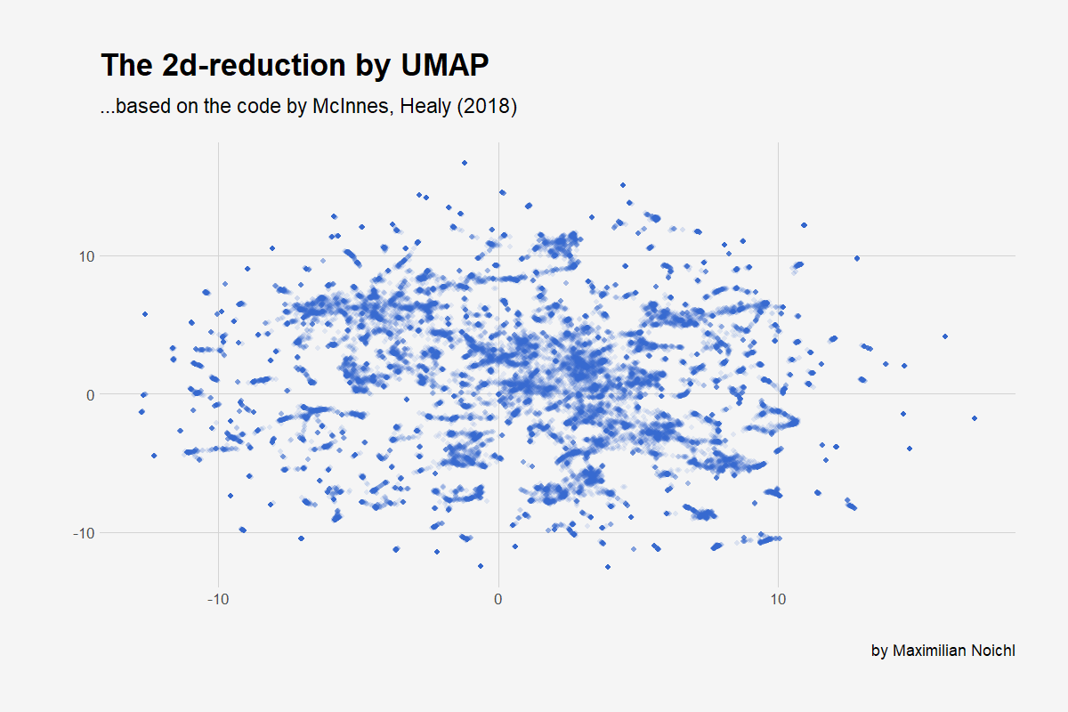
Umap is pretty young technique for dimensionality reduction, which has the big advantage of beeing pretty fast. And it seems to preserve global structure quite reliably, which is nice, as it enables us to cluster afterwards. We will plot the 2D-embedding with ggplot, so that we have something to look at:
|
|
|
|
C:\Users\user\Anaconda3\lib\site-packages\rpy2\robjects\pandas2ri.py:190: FutureWarning: from_items is deprecated. Please use DataFrame.from_dict(dict(items), ...) instead. DataFrame.from_dict(OrderedDict(items)) may be used to preserve the key order.
  res = PandasDataFrame.from_items(items)
Temporal Embedding
Now we will do the same thing we did above, but we will embedd the data just in one dimension and then re-embedd every year in the resulting structure.
|
|
|
|
C:\Users\user\Anaconda3\lib\site-packages\umap_learn-0.3.3-py3.6.egg\umap\spectral.py:229: UserWarning: Embedding a total of 2 separate connected components using meta-embedding (experimental)
|
|
C:\Users\user\Anaconda3\lib\site-packages\rpy2\robjects\pandas2ri.py:190: FutureWarning: from_items is deprecated. Please use DataFrame.from_dict(dict(items), ...) instead. DataFrame.from_dict(OrderedDict(items)) may be used to preserve the key order.
  res = PandasDataFrame.from_items(items)
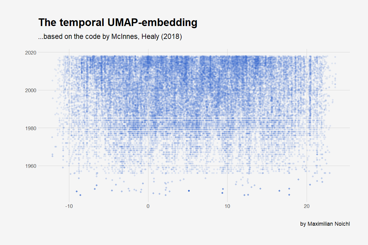
As you can see, the web of science started to archive the months of publishing only in the late eighties, which is why the plot has these lines at the bottom, where we can assign only years to the publications.
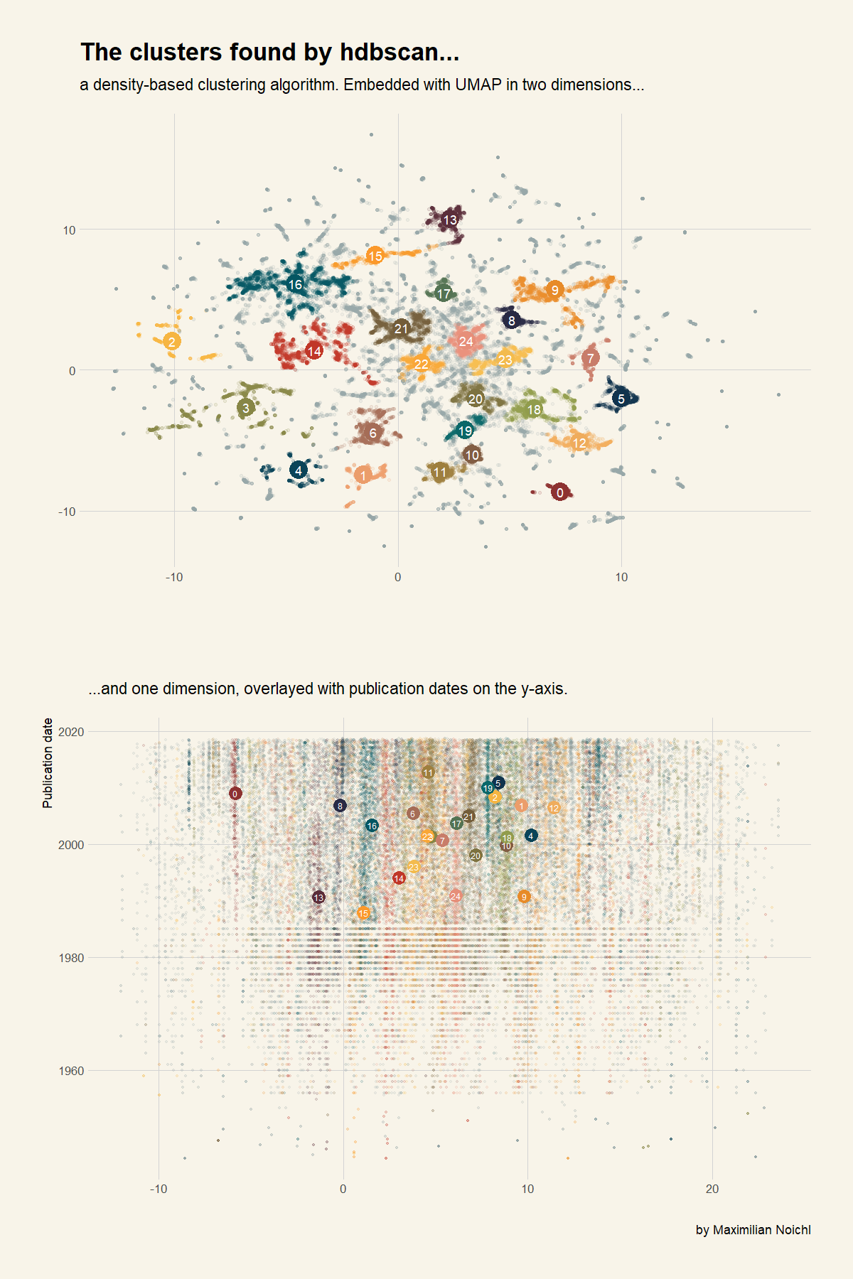
Clustering with HDBSCAN
Now we use HDBSCAN to cluster our data:
|
|
25
Now lets plot everything in ggplot:
|
|
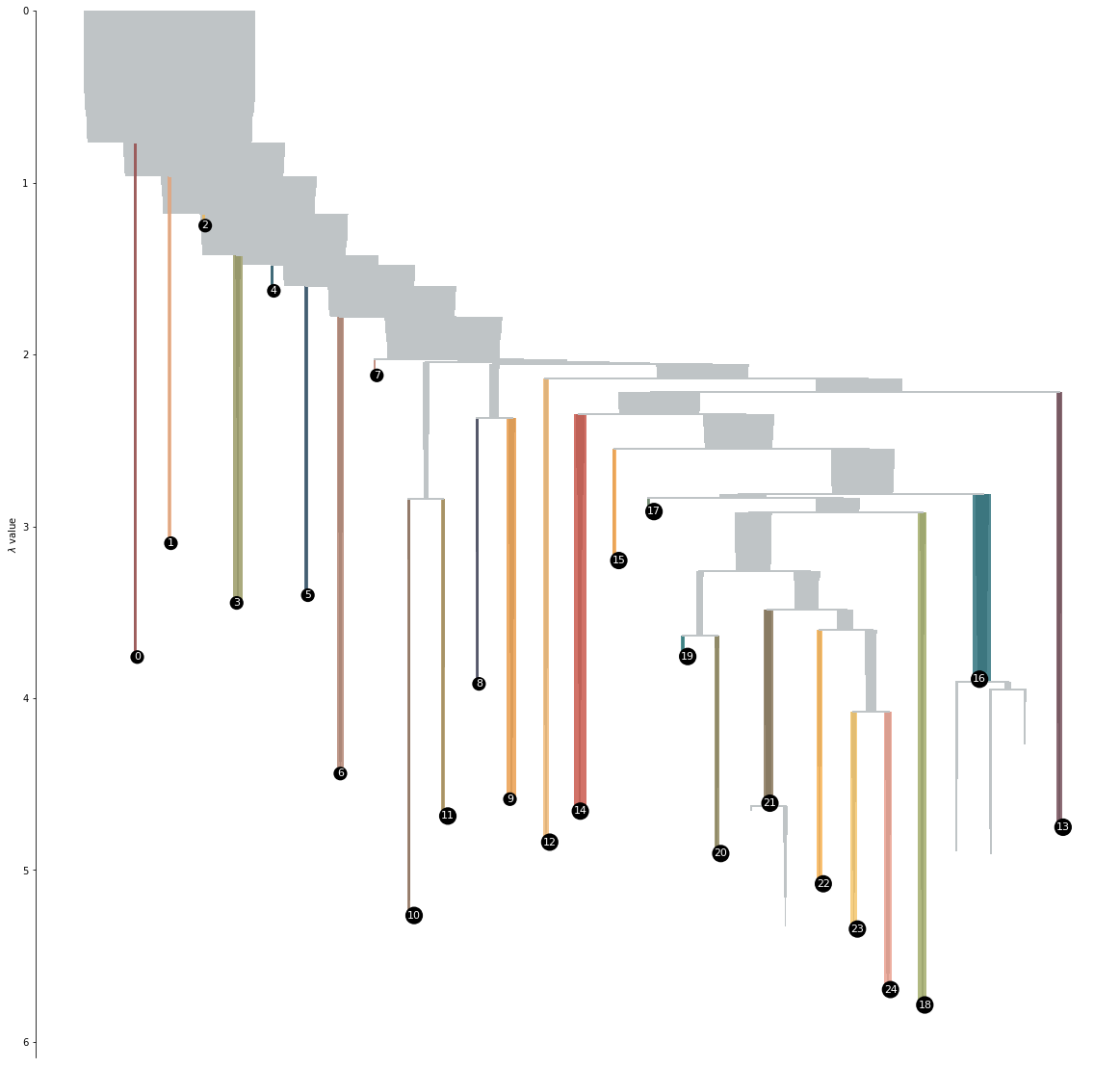
Thats nice. To have look into the way the clustering algorithm has structured the data, lets look at the condensed tree.
I messed around a bit in my installation of HDBSCAN, so if you run this on your computer, your tree will propably look quite different.
The condensed clustering tree basically tells us, when the algorithm found it necessary to break a group apart into two smaller clusters. On the left of the tree we see the clusters that were so far removed from the central structure, that they broke off at the very beginning of the clustering process.
|
|
<matplotlib.axes._subplots.AxesSubplot at 0x18c514a1588>
What does it mean?
Now, let us look into the clusters to find out what they actually contain. First we will analyze the abstracts of the papers in every cluster according to their most common words and bigrams. In the tables below, every column is a cluster, and every row is a common word. Then we will do the exact same thing with the most cited authors.
|
|
|
|
| 0 | 1 | 2 | 3 | 4 | 5 | 6 | 7 | 8 | 9 | 10 | 11 | 12 | 13 | 14 | 15 | 16 | 17 | 18 | 19 | 20 | 21 | 22 | 23 | 24 | |
|---|---|---|---|---|---|---|---|---|---|---|---|---|---|---|---|---|---|---|---|---|---|---|---|---|---|
| 0 | free | logic | coherence | logic | logic | causal | probability | newtons | conditionals | science | justification | knowledge | evolutionary | moral | kants | moral | moral | fictional | cognitive | phenomenal | properties | argument | names | language | language |
| 1 | argument | truth | properties | semantics | logics | explanation | models | theories | causation | quantum | epistemic | epistemic | selection | aristotle | kant | rights | reasons | logic | mental | experience | mental | objects | view | logic | quines |
| 2 | responsibility | logics | confirmation | language | epistemic | explanations | scientific | newton | causal | scientific | belief | belief | evolution | virtue | moral | argument | view | argument | view | consciousness | physical | properties | argument | truth | view |
| 3 | moral | paradox | dispositions | semantic | knowledge | models | evidence | natural | counterfactual | theories | knowledge | argument | species | character | argument | view | argument | fiction | mind | argument | causal | view | semantic | freges | truth |
| 4 | agent | model | analysis | analysis | models | mechanistic | science | mathematics | semantics | explanation | beliefs | view | biological | view | philosophy | problem | normative | aesthetic | states | experiences | problem | modal | reference | wittgensteins | logical |
| 5 | action | classical | measures | set | agents | mechanisms | problem | logic | counterfactuals | mechanics | justified | evidence | natural | ethics | view | claim | reason | problem | content | perceptual | argument | problem | terms | frege | theories |
| 6 | agents | logical | models | natural | model | explanatory | decision | set | conditional | problem | problem | justification | biology | philosophical | human | human | value | view | psychology | view | causation | possible | proper | logical | philosophy |
| 7 | principle | models | measure | model | belief | model | bayesian | theorem | view | understanding | view | assertion | social | nature | nature | life | good | arguments | argument | content | action | time | modal | philosophical | argument |
| 8 | responsible | semantics | laws | context | dynamic | science | argument | philosophy | problem | causal | evidence | problem | concept | aristotles | science | social | problem | semantics | cognition | properties | view | worlds | descriptions | view | logic |
| 9 | determinism | notion | evidence | meaning | finite | scientific | model | new | argument | philosophy | perceptual | know | different | social | does | does | claim | question | theories | states | physicalism | arguments | kind | problem | semantics |
| 10 | does | theories | argument | notion | modal | mechanism | theories | classical | analysis | view | epistemology | cases | kinds | good | reason | order | theories | questions | function | perception | emergence | identity | semantics | argument | carnaps |
| 11 | cases | semantic | robustness | structure | information | different | belief | proof | cases | physical | argument | contextualism | models | knowledge | arguments | people | action | way | language | conscious | actions | way | arguments | wittgenstein | quine |
| 12 | arguments | consequence | nature | interpretation | results | biology | probabilities | analysis | indicative | new | truth | true | genetic | model | natural | morally | way | epistemic | problem | mental | exclusion | world | natural | philosophy | philosophical |
| 13 | problem | modal | dispositional | view | logical | biological | view | mathematical | theories | explanations | conservatism | knows | view | does | way | value | agents | knowledge | systems | physicalism | claim | different | theories | objects | science |
| 14 | claim | paradoxes | view | results | game | causation | new | second | possible | argument | reasons | closure | information | problem | role | way | does | sentences | representations | character | philosophy | true | meaning | terms | semantic |
| 15 | control | paraconsistent | results | argument | language | theories | approach | results | standard | interpretation | true | epistemology | human | explain | terms | theories | practical | true | claim | physical | events | metaphysical | problem | notion | meaning |
| 16 | objection | relevant | causal | logical | result | systems | principle | does | probability | model | memory | does | cultural | human | concept | certain | belief | value | science | concepts | second | parts | belief | conception | scientific |
| 17 | alternative | language | bayesian | different | action | cognitive | epistemic | use | true | elsevier | process | arguments | model | reason | claim | important | arguments | belief | representation | way | davidsons | does | new | sense | knowledge |
| 18 | morally | prove | probabilistic | theories | algebras | view | case | order | truth | explanatory | thesis | beliefs | processes | life | knowledge | justice | rational | information | role | claim | explanation | things | logic | thought | arguments |
| 19 | actions | calculus | problem | new | games | approach | representation | models | particular | philosophical | according | principle | role | way | philosophical | make | certain | different | recent | visual | relation | present | content | use | ontological |
|
|
| 0 | 1 | 2 | 3 | 4 | 5 | 6 | 7 | 8 | 9 | 10 | 11 | 12 | 13 | 14 | 15 | 16 | 17 | 18 | 19 | 20 | 21 | 22 | 23 | 24 | |
|---|---|---|---|---|---|---|---|---|---|---|---|---|---|---|---|---|---|---|---|---|---|---|---|---|---|
| 0 | moral responsibility | classical logic | robustness analysis | natural language | epistemic logic | mechanistic explanation | sleeping beauty | elsevier rights | indicative conditionals | quantum mechanics | epistemic justification | true belief | natural selection | character traits | elsevier rights | combination problem | moral responsibility | fictional characters | cognitive science | phenomenal character | mental causation | possible worlds | proper names | abstraction principles | natural language |
| 1 | morally responsible | sequent calculus | laws nature | firstorder logic | dynamic epistemic | mechanistic explanations | philosophy science | natural philosophy | actual causation | elsevier rights | phenomenal conservatism | knowledge attributions | evolutionary biology | elsevier rights | common sense | decision making | normative reasons | aesthetic value | mental states | perceptual experience | exclusion problem | material objects | natural kind | caesar problem | philosophy science |
| 2 | alternative possibilities | logical consequence | coherence measures | definite descriptions | belief revision | multiple realization | dutch book | explicit mathematics | counterfactual dependence | philosophy science | generality problem | practical reasoning | natural kinds | virtue ethics | practical reason | harm principle | practical reasoning | epistemic logic | social cognition | phenomenal concepts | physical properties | david lewis | definite descriptions | humes principle | ontological commitment |
| 3 | consequence argument | theories truth | bayesian confirmation | valued fields | modal logic | philosophy science | elsevier rights | second order | possible worlds | scientific revolutions | justified belief | knowledge norm | group selection | moral view | human nature | incentives argument | moral judgments | discourse fiction | folk psychology | phenomenal consciousness | mental properties | temporal parts | kind terms | natural language | formal semantics |
| 4 | principle alternative | truth predicate | ceteris paribus | logical form | modal logics | scientific explanation | degrees belief | general relativity | subjunctive conditionals | scientific theories | basing relation | epistemic contextualism | developmental biology | mimetic desire | philosophy science | inner speech | reasons action | fictional entities | natural selection | knowledge argument | causal exclusion | common sense | direct reference | singular terms | indeterminacy translation |
| 5 | free action | paraconsistent logics | conditional analysis | boolean algebras | common knowledge | causal relations | causal decision | action distance | causal claims | measurement problem | perceptual experience | norm assertion | cultural evolution | nicomachean ethics | transcendental idealism | human beings | moral realism | possible worlds | language thought | mental states | philosophy mind | modal realism | possible worlds | philosophy mathematics | philosophy language |
| 6 | manipulation arguments | semantic paradoxes | measures coherence | generalized quantifiers | firstorder logic | elsevier rights | expected utility | reverse mathematics | counterfactual conditionals | wave function | true belief | external world | units selection | emotional disorder | model pa | moral judgments | intrinsic value | fictional realism | mental representation | mental state | emergent properties | states affairs | complex demonstratives | logical objects | scientific theories |
| 7 | argument incompatibilism | liar paradox | dispositional properties | natural deduction | dynamic logic | explanatory power | scientific realism | fixed point | semantics counterfactuals | common cause | gettier problem | gettier cases | evolutionary processes | mechanical problems | categorical imperative | moral luck | moral properties | modal logic | false belief | perceptual experiences | downward causation | impossible worlds | modal logic | julius caesar | analyticsynthetic distinction |
| 8 | free moral | modal logic | measure coherence | logical consequence | kripke models | multiple realizability | scientific representation | does imply | truth conditions | scientific explanation | true beliefs | justified belief | inclusive fitness | moral dilemmas | natural philosophy | ordinary people | practical reasons | negative existentials | mental content | conscious experience | mental states | possible world | attitude ascriptions | philosophical investigations | elsevier rights |
| 9 | van inwagens | logical pluralism | probabilistic measures | subset equal | epistemic logics | causal inference | scientific theories | space time | causal exclusion | interpretation quantum | beliefs justified | perceptual knowledge | evolutionary game | social psychology | natural science | sense embodiment | moral facts | imaginative resistance | mental representations | phenomenal properties | mental physical | time travel | general terms | bad company | common sense |
| 10 | direct argument | relevant logics | analysis dispositions | truth conditions | public announcements | case study | van fraassen | classical mechanics | ramsey test | philosophers science | doxastic justification | pragmatic encroachment | population genetics | undecidable problems | pure reason | absolute margin | practical reason | natural language | philosophy mind | explanatory gap | nonreductive physicalism | ordinary objects | freges puzzle | plural logic | grellings paradox |
| 11 | alternate possibilities | relevance logic | confirmation measures | greater equal | action models | molecular biology | scientific practice | order arithmetic | david lewiss | explanatory power | epistemic status | transmission failure | tree life | absolute goodness | space time | duty vote | public reason | paradox fiction | cognitive architecture | naive realism | causal powers | david lewiss | singular thought | symmetric godel | language learning |
| 12 | possibilities pap | sequent calculi | conjunction fallacy | scalar implicatures | boolean games | causal explanation | beauty problem | seventeenth century | david lewis | scientific knowledge | inferential justification | epistemic closure | niche construction | character trait | death penalty | human dignity | moral discourse | seeing things | cognitive neuroscience | representational content | problem mental | negative truths | definite description | godel logic | natural kinds |
| 13 | principle alternate | strong kleene | categorical properties | quantifier elimination | cylindric algebras | cognitive science | book arguments | natural numbers | epistemic modals | scientific realism | justified beliefs | epistemic luck | philosophy biology | concept character | eighteenth century | invisible hand | political liberalism | fictional names | jerry fodor | phenomenal content | mental events | proper parts | semantic value | philosophical problems | ontological categories |
| 14 | frankfurt cases | propositional logic | degree coherence | real closed | et al | causal markov | quantum mechanics | ramseys theorem | theories causation | elsevier science | justified believing | concept knowledge | species concepts | evaluational internalism | human rights | legal punishment | virtue ethics | category mistakes | nonhuman animals | visual experience | intentional action | composition identity | singular terms | abstract objects | conceptual realism |
| 15 | agent morally | relevant logic | reliability conducive | boolean algebra | expressive power | markov condition | van fraassens | recursive functions | structural equations | scientific practice | regress problem | doxastic justification | evolutionary developmental | john doris | incompleteness theorem | moral concern | rational requirements | classical logic | propositional attitudes | conscious states | donald davidsons | modal logic | rigid designation | alethic functionalism | indeterminacy thesis |
| 16 | agent causation | truth values | possible worlds | linear logic | predicate logic | biological sciences | case study | theorem pairs | causal decision | case study | thought experiment | knowledge ascriptions | multilevel selection | moral behaviour | kants argument | moral conflict | moral error | classical music | representational content | concept strategy | exclusion argument | properties relations | rigid designators | alethic pluralism | language acquisition |
| 17 | compatibilists incompatibilists | yablos paradox | probabilistic coherence | semantic analysis | temporal logic | causal structure | subjective probability | classical logic | causal explanation | science rights | belief justified | closure principle | social sciences | moral virtue | constitutive rules | moral virtue | moral judgements | fictional discourse | cognitive processes | phenomenal concept | jaegwon kim | argument vagueness | view names | cardinal numbers | logical consequence |
| 18 | determinism true | paraconsistent logic | finks masks | algebraically closed | van benthem | philosophers science | probability function | experimental philosophy | conditional probabilities | causal processes | perceptual beliefs | knowledge assertion | species concept | prima facie | critique pure | notion social | practical rationality | figurative language | cognitive systems | philosophy mind | prima facie | abstract objects | mental states | oxford university | logical truths |
| 19 | perform action | modal logics | austere quidditism | categorial grammar | announcement logic | constitutive relevance | philosophers science | firstorder logic | modus ponens | configuration space | process reliabilism | epistemic value | recent work | problem evil | early modern | able explain | reasons belief | gods existence | connectionist models | hard problem | causal closure | bare particulars | modal epistemology | person authority | principle charity |
|
|
| 0 | 1 | 2 | 3 | 4 | 5 | 6 | 7 | 8 | 9 | 10 | 11 | 12 | 13 | 14 | 15 | 16 | 17 | 18 | 19 | 20 | 21 | 22 | 23 | 24 | |
|---|---|---|---|---|---|---|---|---|---|---|---|---|---|---|---|---|---|---|---|---|---|---|---|---|---|
| 0 | fischer | anderson | armstrong | barwise | hughes | craver | jeffrey | friedman | lewis | popper | goldman | williamson timothy | hull | aristotle | kant | nozick | rawls | walton | fodor | tye | davidson | lewis | kripke | wittgenstein | quine |
| 1 | mele | priest | lewis | chang | van benthem | woodward | hacking | newton | stalnaker | hempel | alston | cohen | sober | plato | smith | feinberg | williams | plantinga | churchland | chalmers | kim | armstrong | salmon | dummett | davidson |
| 2 | frankfurt | belnap | martin | bach | fagin | cartwright | lewis | earman | lewis david | kuhn | chisholm | hawthorne | wilson | ross | hume | mill | scanlon | hintikka | dennett | dretske | davidson donald | lewis david | kaplan | frege | carnap |
| 3 | van inwagen peter | beall | ellis | partee | halpern | bechtel | van fraassen | church | adams | salmon | pollock | derose | lewontin | cooper | locke | rawls | parfit | lewis | millikan | block | lewis | sider | lewis | wright | russell |
| 4 | pereboom | dunn | bird | tarski | baltag | machamer | giere | feferman | bennett | feyerabend | bonjour | dretske | gould | irwin | kant immanuel | hare | nagel | kripke | dretske | jackson | mele | quine | soames | wright crispin | putnam |
| 5 | kane robert | meyer | fitelson | lewis | gabbay | wimsatt | savage | simpson | hitchcock | kuhn thomas | lehrer | lewis | mayr | none | none | nagel thomas | hare | currie | cummins | dennett | fodor | kripke | donnellan | kripke | quine wvo |
| 6 | ginet | kripke | mumford | kamp | van ditmarsch | fodor | levi | cohen | jackson | einstein | harman | goldman | dawkins | aquinas | husserl | hart | cohen | currie gregory | goldman | byrne | goldman | fine | perry | frege gottlob | goodman |
| 7 | strawson | field | olsson | dowty | blackburn | glennan | kyburg | troelstra | edgington | reichenbach | sosa | sosa | smith | vlastos | strawson | none | rawls john | vaninwagen | searle | lycan | horgan | van inwagen | evans | dummett michael | kripke |
| 8 | kane | routley | bird alexander | heim irene | segerberg | kim | vanfraassen | kreisel | woodward | bell | bonjour laurence | pritchard | griffiths | hett | goodman | dworkin | none | carroll | putnam | armstrong | wilson | merricks | burge | wittgenstein ludwig | strawson |
| 9 | widerker | restall | molnar | heim | troelstra | schaffner | howson | westfall | schaffer | lakatos | dretske | williamson | sterelny | nussbaum | aristotle | williams | gibbard | salmon | stich | harman | searle | lowe | putnam | strawson | frege |
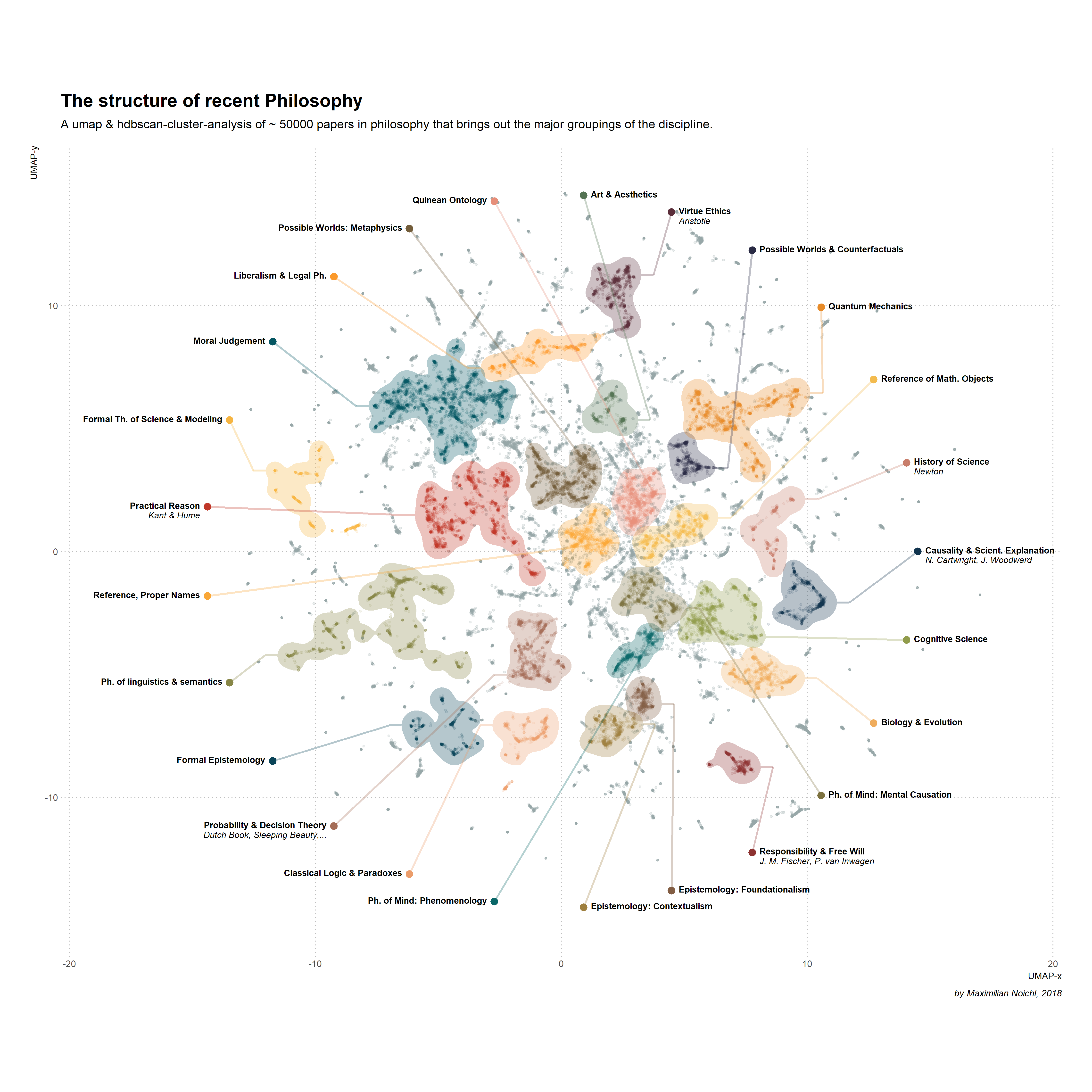
Now for the final part that puts it all together into a labeled graph. Note that the labels are my interpretation and reasonable people can very well disagree about them.
|
|
And Voilà! here we have the graphic from the beginning.
Author Maximilian Noichl
LastMod 2018-09-15