0.1 Widom's technique and Nezbeda-Kolafa's extension

The basic idea of the Widom test particle method is to try to insert, at regular intervals, a particle at a random position. The particle is assumed to have no influence on the rest of the system, but it has an energy $\Delta U_{t} \equiv U_{N+1}-U_{N}$ with respect to the $N$ ``real'' particles. From

$$\exp[-\beta \mu_{r}] = \exp[-\beta (A_{N+1}-A_{N}) ] = ... ...N}\exp[-\beta U_{N}] } = <\exp[-\beta \Delta U_{t}]>_{N}$$ (1)

(with $\mu_{r}=\mu-\mu_{id}$) we conclude that

$$\exp[-\beta \mu]=Q_{id} <\exp[-\beta \Delta U_{t}]>_{N}$$ (2)

In a MC or MD simulation, then, we periodically try to introduce a visiting particle and register its Boltzmann factor $\exp[-\beta \Delta U_{t}]$ for averaging.

Evidently, in a dense system the addition of another particle at a random position will result in a very low Boltzmann factor of that particle. Thus a lot of almost-zeroes will be added up for averaging.

A gradual insertion, or ``staging'' (Kofke) method may help to improve the efficiency. The first implementation of such a technique is due to Mon and Griffiths (1985). In Nezbeda and Kolafa's work (1991) this older version is dubbed ``method A'' while their own modification is called method B.

Method A: Write the ratio $Q_{N+1}/V Q_{N+1}$ as

$$\frac{Q_{N+1}}{V Q_{N}} = \frac{Q_{N+\sigma_{1}}}{Q_{N}} \... ...igma_{1}}} \dots \frac{Q_{N+\sigma_{k}}}{Q_{N+\sigma_{k-1}}}$$ (3)

where $\sigma_{k} \equiv \sigma$ and $\sigma_{i}\; (i=1, \dots k-1)$ pertains to an intermediate state of a scaled particle. Thus

$$\frac{Q_{N+1}}{V Q_{N}} = <\exp[-\beta \Delta U_{N+\sig... ...\sigma_{i}}]>_{N+\sigma_{i}} = q_{0} \prod_{i=1}^{k-1} q_{i}$$ (4)

In method A each of the factors $<\exp[-\beta \Delta U_{N+\sigma_{i+1}}-U_{N+\sigma_{i}}]>_{N+\sigma_{i}}$ is determined in a separate simulation, so that $k$ simulations are needed to arrive at an estimate of $\mu$.

Method B: Nezbeda and Kolafa suggested that one long MC run be used to sample all intermediate and final states of the generalized ensemble made up of $N+\sigma_{i}$ particles. The tentative growing or shrinking of a particle is then just another one of the MC trial steps. Assigning weights $w_{i}$ to the various sub-ensembles, the Monte Carlo transition probability is

$$P_{i \rightarrow j} = {\rm min} \left\{ 1, \frac{p_{ij}}{p... ...w_{j} \exp[-\beta U_{j}]}{w_{i} \exp[-\beta U_{i}]}\right\}$$ (5)

where the $p_{ij}$ ($j=i-1$ or $i+1$) are the a priori trial probabilities for growing and shrinking. The optimal choice for the weights $w_{i}$ and $p_{ij}$ are considered below.

The residual chemical potential is given by

$$\beta \mu_{r} = \ln \left[ w_{k} Pr(N)/Pr(N+1)\right]$$ (6)

with $Pr(N)$ the probability (or relative frequency) of state $N$ in the semi-grand ensemble spanned by all states of the systems $\{ N, N+\sigma_{1} \dots N+1\}$.

Method C: As a further generalization, Nezbeda and Kolafa consider the grand canonical ensemble spanned by $\{ 0, 0+\sigma_{1}, \dots N, N+\sigma_{1}, \dots N+1, \dots \infty \}$. We will not treat this any further.



Optimal parameters: The growing of particles by one size stage should be equally probable for all $i$. Taking hard spheres as an example, the chemical potential for $\sigma_{i} \rightarrow \sigma_{i+1}$ is approximately proportial to $\sigma_{i}^{2}$. Therefore, the hard sphere diameter should be discretized according to $\sigma_{i}=\sqrt{i/k} \sigma$. Other coupling parameters than the particle diameter may be treated in a similar way.

The best choice for the weights $w_{i}$ is $w_{i+1}/w_{i}=\exp[\beta \mu_{r}/k]$.

For best performance, the trial probabilities $p_{ij}$ should be such that $w_{j} p_{ji}=w_{i} p_{ij}$ (see 5). For the first stage, $N \rightarrow N+\sigma_{1}$ we take this probability as $=1$, and for the intermediate steps $i=2,3, \dots k-1$ we have $p_{i,i+1}=1-p_{i-1,i} \exp[-\beta \mu_{r}/k]$. At the final step, there is no further growth, and the non-change is tried with probability $p_{N+1,N+1} = 1-p_{N+\sigma_{k-1},N+1}\exp[-\beta \mu_{r}/k]$. At all stages, the sum of the two trial probabilities equals $1$. (In the grand canonical method C, the rules are slightly more symmetric, since a growth beyond $N+1$ and a shrinkage below $N$ is permitted.)

Test of the method by Nezbeda/Kolafa:
These authors chose a HS fluid as their test sample. The chemical potential in this case may be calculated explicitely by integrating the Carnahan-Starling formula:

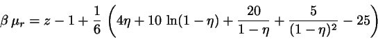$$\beta \mu_{r}= z-1+\frac{1}{6} \left( 4 \eta + 10 \ln(1-\eta) + \frac{20}{1-\eta} +\frac{5}{(1-\eta)^{2}}-25\right)$$ (7)

with $z=\left( 1+\eta+\eta^{2}-(2/3)(\eta^{3}+\eta^{4})\right)/(1-\eta)^{3}$. Thus the simulation results may be checked against (semi-)exact theory.

[to be extended...]