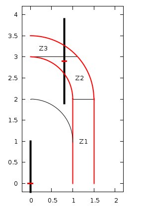
Square Well Lines

Parallel (par):
Let the center of particle 1 be the origin of a cylindrical coordinate system, with particle 2 sitting at $(\rho, z)$. Considering only positive values of z, we find for the following ranges for $\rho$:

$ \begin{eqnarray} {\rm Region \; Z1:}\; z \, \varepsilon \, [ 0, 2h] \;\;\; && \rightarrow \;\;\; \rho \, \varepsilon \, \left[ 1, r_{2} \right] \\ {\rm Region \; Z2:}\; z \, \varepsilon \, [ 2h, 2h+1) \;\;\; && \rightarrow \;\;\; \rho \, \varepsilon \, \left[ \sqrt{1-(z-2h)^{2}}, \sqrt{r_{2}^{2}-(z-2h)^{2}} \right] \\ {\rm Region \; Z3:}\; z \, \varepsilon \, [ 2h+1, 2h+r_{2} ] \;\;\; && \rightarrow \;\;\; \rho \, \varepsilon \, \left[ 0, \sqrt{r_{2}^{2}-(z-2h)^{2}} \right] \end{eqnarray} $

The following applies in all of these regions.
Given a position $\rho, z$ and a pair of internal points $\gamma, \delta$ we demand that $s^{2} \equiv \rho^{2}+ (z+\delta - \gamma )^{2}$ be smaller than $r_{2}$. For any given $\gamma$ this sets limits for $\delta$, which are the solutions of $ \delta^{2}+2\delta (z-\gamma )+(z-\gamma )^{2} - a^{2} = 0 $ where $a^{2}=r_{2}^{2}-\rho^{2}$. These solutions are $\delta = -(z-\gamma ) \pm a$. In other words, we have

$ \delta_{min} = \max [-h,\! -\!(z\!-\!\gamma )\! -\! a] \;\;\;\; \delta_{max} = \min [ h, \!-\!(z\!-\!\gamma )\! +\! a] $

For the extreme values of $\delta = \pm h$ we find four respective limiting values of $\gamma \,$:

$ \begin{eqnarray} \gamma_{1}&=& \min(h,\max(\!-\!h,z\!-\!h\!-\!a)) \;\;\;\; \gamma_{2}= \min(h,\max(\!-\!h,z\!+\!h\!-\!a)) \\ \gamma_{3}&=& \max(-h,\min( h,z\!-\!h\!+\!a)) \;\;\;\; \gamma_{4}= \max(-h,\min( h,z\!+\!h\!+\!a)) \end{eqnarray} $

Depending on the relative sizes of $\gamma_{2}$ and $\gamma_{3}$ we discern two cases:

Case 1: $\gamma_{2} \leq \gamma_{3}$:

$ \begin{eqnarray} u(1,2) & = & \frac{\textstyle - \epsilon }{\textstyle L^{2}} \left[ \int \limits_{\textstyle \gamma_{1}}^{\textstyle \gamma_{2}} d \gamma \, [ \, h \! + \! a \! - \! z \! + \! \gamma \, ] + \, 2 h \int \limits_{\textstyle \gamma_{2}}^{\textstyle \gamma_{3}} d \gamma \, +\int \limits_{\textstyle \gamma_{3}}^{\textstyle \gamma_{4}} d \gamma \, [ \, h \! + \! a \! + \! z \! - \! \gamma \, ] \right] \\ & = & \\ & = & \frac{\textstyle - \epsilon }{\textstyle L^{2}} \left[ ( h \! + \! a \! - \! z )( \gamma_{2} \! - \! \gamma_{1} ) \! + \! ( \gamma_{2}^{2} \! - \! \gamma_{1}^{2} ) / 2 \! + \! 2 h \, ( \gamma_{3} \! - \! \gamma_{2} ) \! + \! ( h \! + \! a \! + \! z )( \gamma_{4} \! - \! \gamma_{3} ) \! - \! ( \gamma_{4}^{2} \! - \! \gamma_{3}^{2} ) / 2 \right] \end{eqnarray} $

Case 2: $\gamma_{2} > \gamma_{3}$:

$ \begin{eqnarray} u(1,2) & = & \frac{\textstyle - \epsilon }{\textstyle L^{2}} \left[ \int \limits_{\textstyle \gamma_{1}}^{\textstyle \gamma_{3}} d \gamma \, [ \, h \! + \! a \! - \! z \! + \! \gamma \, ] + \, 2 a \int \limits_{\textstyle \gamma_{3}}^{\textstyle \gamma_{2}} d \gamma \, +\int \limits_{\textstyle \gamma_{2}}^{\textstyle \gamma_{4}} d \gamma \, [ \, h \! + \! a \! + \! z \! - \! \gamma \, ] \right] \\ & = & \\ & = & \frac{\textstyle - \epsilon }{\textstyle L^{2}} \left[ ( h \! + \! a \! - \! z )( \gamma_{3} \! - \! \gamma_{1} ) \! + \! ( \gamma_{3}^{2} \! - \! \gamma_{1}^{2} ) / 2 \! + \! 2 a \, ( \gamma_{2} \! - \! \gamma_{3} ) \! + \! ( h \! + \! a \! + \! z )( \gamma_{4} \! - \! \gamma_{2} ) \! - \! ( \gamma_{4}^{2} \! - \! \gamma_{2}^{2} ) / 2 \right] \end{eqnarray} $

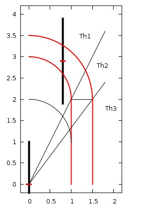
Figure 1: Square well lines, parallel, $L=2$, $r_{2}=1.5$; z=0 to z=2.0 - i.e. region Z1.

Figure 2: Square well lines, parallel, $L=2$, $r_{2}=1.5$; z=2.0 to z=3.4 - i.e. regions Z2-Z3.

Alternatively, we may describe the pair in polar coordinates $(r, \theta)$.

Three regions for $\theta$:

$ \begin{eqnarray} \Theta 1: \; \theta \, \varepsilon \, [ 0 \, , \, \arctan 1/2h] \;\;\; & \rightarrow & \;\;\; r \, \varepsilon \, \left[ 2 h \cos \theta + \sqrt{1-4 h^{2} \sin^{2} \theta } \, , \, 2 h \cos \theta + \sqrt{r_{2}^{2}-4 h^{2} \sin^{2} \theta } \right] \\ \Theta 2: \; \theta \, \varepsilon \, [ \arctan 1/2h \, , \, \arctan r_{2} /2h] \;\;\; & \rightarrow & \;\;\; r \, \varepsilon \, \left[ 1 / \sin \theta \, , \, 2 h \cos \theta + \sqrt{r_{2}^{2}-4 h^{2} \sin^{2} \theta } \right] \\ \Theta 3: \; \theta \, \varepsilon \, [ \arctan r_{2} /2h \, , \, \pi/2 ] \;\;\; & \rightarrow & \;\;\; r \, \varepsilon \, \left[ 1 / \sin \theta \, , \, r_{2} / \sin \theta \right] \end{eqnarray} $

Figure 3: Square well lines, parallel, $L=2$, $r_{2}=1.5$; $\theta = 0$ to $0.4 \cdot \pi/2$ - i.e. regions $\Theta 1$ - $\Theta 2$.

Figure 4: Square well lines, parallel, $L=2$, $r_{2}=1.5$; $\theta = 0.4 \cdot \pi/2$ to $\pi/2$ - i.e. region $\Theta 3$.

Square Well Lines / Parallel case