Square Well Lines (SWL):
General (non-parallel) configuration
Model suggested by Szabolcs Varga, Oct 2008:
Consider two lines of finite length $L = 2h$ containing a homogeneous
density of square well centers.
Let $\vec{e}_{1,2}$ be the direction vectors,
$\vec{r}_{12}$ the vector between the centers of the two line
segments, and $\lambda, \, \mu$ parameters giving the positions of
the interacting points along $1$ and $2$. The squared distance between
any two such points is given by
$r^{2}= \left|
r_{12}+\mu \cdot \vec{e}_{2}-\lambda \cdot \vec{e}_{1}
\right|^{2}
$.
The total interaction energy between the two lines is then
$
u(1,2) \equiv u(\vec{r}_{12},\vec{e}_{1},\vec{e}_{2}) =
\frac{\textstyle 1}{\textstyle L^{2}}
\int \limits_{\textstyle 1}d\lambda \int \limits_{\textstyle 2}d\mu \, \,
u_{SW}\left[ r(\lambda,\mu) \right]
$
with $u_{SW}(r)= \infty $ if $r < 1$, $= - \epsilon $
if $1 < r < r_{2}$, and $=0$ for $r > r_{2}$. Typically,
$r_{2}=1.5 - 2.0$.
Any 2d configuration (except $d=1$):
Having found the intersection point $(\lambda_{0},\mu_{0})$ of
the carrier lines on which the two sticks reside, we move the
coordinate origin to this point. The centers of the two sticks are
then at $\gamma_{0}=-\lambda_{0}$, $\delta_{0}=-\mu_{0}$.
Written in the new coordinates the potential is
$
u(1,2) \equiv u(\vec{r}_{12},\vec{e}_{1},\vec{e}_{2}) =
\frac{\textstyle - \epsilon}{\textstyle L^{2}}
\int \limits_{\textstyle \gamma_{0}-h}^{\textstyle \gamma_{0}+h} d \gamma
\int \limits_{\textstyle \delta_{0}-h}^{\textstyle \delta_{0}+h} d \delta \, \,
u_{SW}\left[ r(\gamma, \delta) \right]
$
with
$r^{2}(\gamma, \delta) = \gamma^{2}+\delta^{2}-2 \gamma \delta d$.
In the $(\gamma, \delta )$ plane the integration region is
represented by a square $S$ of side length $L$ around
$(\lambda_{0},\mu_{0})$. However, the integrand in non-zero,
and constant, only for $ r^{2}(\gamma, \delta ) < r_{2}^{2}$.
In other words, the integral gives the area shared by the square
$S$ and an ellipse $E$ described by
$\gamma^{2}+\delta^{2}-2 \gamma \delta d -r_{2}^{2}=0$.
|
The potential between two SWL particles is given by
the area of the overlap region between the square
$S: \{ \gamma_{0} \pm h, \delta_{0} \pm h, \}$
and the ellipse
$E: \gamma^{2}+\delta^{2}-2 \gamma \delta d -r_{2}^{2}=0$
.
|
Since this overlap
region must be within the smallest rectangle $R$ containing the
ellipse, only the - generally rectangular - section
$S \cap R$
needs to be considered; see Fig. 1.
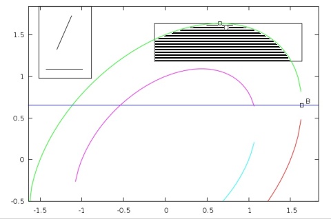 Figure 1:
Square well lines: $L=2$, $r_{2}=1.5$. The inset shows the configuration
represented in the $\gamma, \delta$ plane. The potential is given by
the overlap area of square and ellipse. The horizontal line through
the rightmost ellipse point is important for discriminating 3 cases
(see text.) [Ignore the gaps in the ellipse - just bad use of gnuplot...]
Figure 1:
Square well lines: $L=2$, $r_{2}=1.5$. The inset shows the configuration
represented in the $\gamma, \delta$ plane. The potential is given by
the overlap area of square and ellipse. The horizontal line through
the rightmost ellipse point is important for discriminating 3 cases
(see text.) [Ignore the gaps in the ellipse - just bad use of gnuplot...]
Here is the procedure in detail:
Consider two sticks in the plane, with centers at $ \vec{r}_{i}$
and with direction vectors $\vec{e}_{i}$ ($i=1,2$). Make sure that
$d \equiv \vec{e}_{1} \cdot \vec{e}_{2} > 0$, if need be by
$\vec{e}_{2} \rightarrow -\vec{e}_{2} $. The rod half length
is denoted by $h \equiv L/2$, and the parameters of points
on the carrier lines, as counted from the rod centers, are
$\lambda$, $\mu$.
We assume that there is no hard body overlap between the two
spherocylinders defined by the repulsive part of the SW
interaction; this may be ascertained in the usual way,
see
here.
-
Determine the intersection of the two carrier lines according
to $\lambda_{0}=(c-bd)/(1-d^{2})$ and $\mu_{0}=(cd-b)/(1-d^{2})$,
with $b \equiv \vec{r}_{12} \cdot \vec{e}_{2}$ and
$c \equiv \vec{r}_{12} \cdot \vec{e}_{1}$.
Using new parameters $\gamma \equiv \lambda - \lambda_{0}$,
$\delta \equiv \mu - \mu_{0}$ originating at the intersection
point we may write the SWL potential as
$
u(1,2) \equiv u(\vec{r}_{12},\vec{e}_{1},\vec{e}_{2}) =
\frac{\textstyle 1}{\textstyle L^{2}}
\int \limits_{\textstyle \gamma_{0}-h}^{\textstyle \gamma_{0}+h} d \gamma
\int \limits_{\textstyle \delta_{0}-h}^{\textstyle \delta_{0}+h} d \delta
\, \,
u_{SW}\left[ r(\gamma, \delta) \right]
$
with
$r^{2}(\gamma, \delta) = \gamma^{2}+\delta^{2}-2 \gamma \delta d$,
and
$u_{SW}(r)/ \epsilon=
\Theta [1 - r]- \Theta [r_{2}-r]$.
We use symmetry arguments to reduce the set of possible pair
configurations $(\gamma_{0},\delta_{0})$:
if $\delta_{0} < 0$ and $\gamma_{0}^{2} < \delta_{0}^{2}$
(lower quadrant),
let $(\gamma_{0},\delta_{0}) \rightarrow (-\gamma_{0},-\delta_{0})$
if $\gamma_{0} > 0$ and $\delta_{0}^{2} < \gamma_{0}^{2}$
(right quadrant),
let $(\gamma_{0},\delta_{0}) \rightarrow (\delta_{0},\gamma_{0})$
if $\gamma_{0} < 0$ and $\delta_{0}^{2} < \gamma_{0}^{2}$
(left quadrant),
let $(\gamma_{0},\delta_{0}) \rightarrow (-\delta_{0},-\gamma_{0})$
The resulting configuration is in the upper quadrant and has the
same overlap integral as the given pair.
-
The rightmost point $B$ and the uppermost point $D$ of
the ellipse
$\gamma^{2}+\delta^{2}-2 \gamma \delta d -r_{2}^{2} = 0 \,$
are given by
$\gamma_{B} = r_{2}/ \sqrt{1-d^{2}}\,$,
$\delta_{B} = d \, \gamma_{B}\,$ and
$\delta_{D} = r_{2}/ \sqrt{1-d^{2}}\,$,
$\gamma_{D} = d \, \delta_{D}\,$.
The relevant integration region is therefore restricted
to the rectangle
$
\begin{eqnarray}
\gamma_{l} & = & \min(\gamma_{0}-h, \gamma_{B}) \, ,
\;\;\;\;
\delta_{l} = \min(\delta_{0}-h, \delta_{D}),
\\
\gamma_{u} & = & \min(\gamma_{0}+h, \gamma_{B}) \, ,
\;\;\;\;
\delta_{u} = \min(\delta_{0}+h, \delta_{D})
\end{eqnarray}
$
-
Determine the left and right intersection points $1,2$ and
$3,4$ of the horizontal rectangle sides with the ellipse.
If such an intersection point is outside the
limits of the respective rectangle side, it is placed at
the near end of that side:
$
\begin{eqnarray}
\gamma_{1} & = & \, \min \left[\gamma_{u}\, , \, \max \left(
d \, \delta_{l} - \sqrt{r_{2}^{2}-\delta_{l}^{2}(1-d^{2})}\, , \, \gamma_{l}
\right) \right]
\\
\gamma_{2} & = & \, \min \left[\gamma_{u}\, , \, \max \left(
d \, \delta_{l} + \sqrt{r_{2}^{2}-\delta_{l}^{2}(1-d^{2})}\, , \, \gamma_{l}
\right) \right]
\\
\gamma_{3} & = & \, \min \left[\gamma_{u}\, , \, \max \left(
d \, \delta_{u} - \sqrt{r_{2}^{2}-\delta_{u}^{2}(1-d^{2})}\, , \, \gamma_{l}
\right) \right]
\\
\gamma_{4} & = & \, \min \left[\gamma_{u}\, , \, \max \left(
d \, \delta_{u} + \sqrt{r_{2}^{2}-\delta_{u}^{2}(1-d^{2})}\, , \, \gamma_{l}
\right) \right]
\\
\end{eqnarray}
$
-
Depending on $\delta_{l}$ and $\delta_{u}$,
the potential $u(\vec{r}_{12},\vec{e}_{1},\vec{e}_{2})$
is now given by:
if $\delta_{u} > \delta_{B}$, $\delta_{l} > \delta_{B}\,$ :
$ u = - \frac{\textstyle \epsilon}{\textstyle L^{2}} \,
( J_{1u}-J_{2u}-J_{34}+M)$
if $\delta_{u} > \delta_{B}$, $\delta_{l} \leq \delta_{B} \,$ :
$ u = - \frac{\textstyle \epsilon}{\textstyle L^{2}} \,
( J_{1u}+J_{2u}-J_{34}+M )$
if $\delta_{u} \leq \delta_{B}$, $\delta_{l} \leq \delta_{B} \,$:
$ u = - \frac{\textstyle \epsilon}{\textstyle L^{2}} \,
( J_{1u}+J_{2u}-J_{34}-2 J_{4u}+M )$
with
$
\begin{eqnarray}
J_{ab} & \equiv &
\int \limits_{\textstyle \gamma_{a}}^{\textstyle \gamma_{b}}
d \gamma \, \sqrt{r_{2}^{2}-\gamma^{2} (1-d^{2})}
= \frac{\textstyle 1}{\textstyle 2 \sqrt{1-d^{2}}}
\left(
\gamma \sqrt{1-d^{2}} \sqrt{r_{2}^{2}-\gamma^{2} (1-d^{2}) }
+r_{2}^{2} \arcsin
\frac{\textstyle \gamma \sqrt{1-d^{2}}}{\textstyle r_{2}}
\right)_{\textstyle \gamma_{a}}^{\textstyle \gamma_{b}}
\\
K_{ab} & \equiv &
\frac{\textstyle 1}{\textstyle 2}
\left(
\gamma_{b}^{2}-\gamma_{a}^{2}
\right)\, , \;\;\;\;
L_{12} \equiv
\delta_{l} (\gamma_{2}-\gamma_{1})\, , \;\;\;\;
L_{34} \equiv
\delta_{u} (\gamma_{4}-\gamma_{3})
\end{eqnarray}
$
and $M \equiv K_{12}-L_{12}-K_{34}+L_{34}$.
|
... but what does it look like?
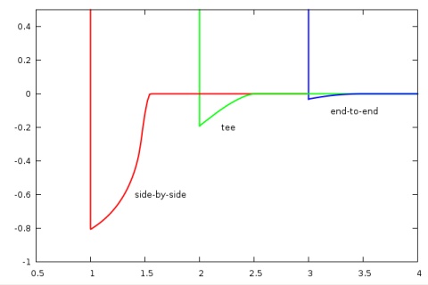 Figure 2: SWL potential as a function of distance for selected orientations.
Compare to LJL
Figure 2: SWL potential as a function of distance for selected orientations.
Compare to LJL
Interestingly, the 3rd dimension will not add to the complexity.
The parameter $r_{2}^{2}$ will simply reduce to
$r_{2}^{2}-r_{0}^{2}$, where $r_{0}$ is the minimum distance between
the carrier lines - at the "proxy points"
$\lambda_{0}$, $\mu_{0}$.
The only remaining problem is the parallel case: so far I have found
no way to express it as a limiting case of a general algorithm;
instead, I always have to treat it separately whenever
$d^{2}>0.9999$ or so.
See here.
Franz Vesely, nov-2008
|
