4.3.1 Constraint dynamics with one bond length
constraint
Molecular Dynamics for Linear Diatomics:
Constraint method
The classical method to simulate diatomics is due to Singer
(1977) and Fincham (1984), as also described in Allen-Tildesley,
Computer Simulation of Liquids (Clarendon, Oxford 1987).
However, we prefer to use the method of ``Constraint Dynamics''
- which is particularly simple when applied to one single constraint.
Assume a diatomic with potential forces acting
on the two atoms, respectively, and write
etc. The only constraint is
.
The equations of motion are then
(4.6)
(4.7)
True to the idea of constraint dynamics, proceed as follows:
Given the positions
at time , integrate the
equations of motion for one time step only considering the
potential forces. The resulting positions are denoted
.
These preliminary position vectors will not fulfill the constraint equation;
rather, the value of
will
be non-zero.
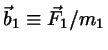
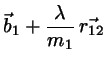
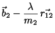
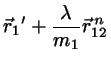
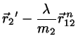
Making the correction ansatz
(4.8)
(4.9)
with undetermined , requiring that the corrected positions
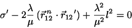
fulfill the constraint equations we find
(4.10)
with
.
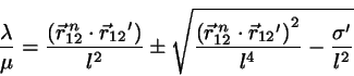
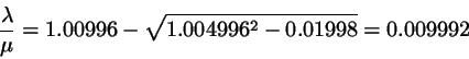
This equation for may be solved exactly:
(4.11)
where the negative sign prevails.
Simple example: Free rotation of a 2D dumbbell
For this problem the constraint method should be exact, since
neither the Verlet propagator nor the constraint reconstruction
introduce errors.
At let
,
;
the masses are
, the angular velocity is , and a time step
of is assumed. Then the exact positions at time
are
(4.12)
and
(4.13)
where we have written
and
.
Now let us test the constraint dynamics procedure against this exact result.
For the Verlet integrator we need
, for which
we take the exact values
and
.
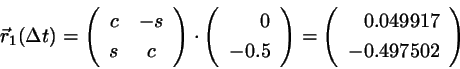
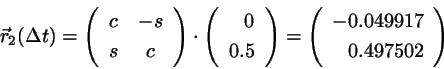
After the free flight the new positions are
(4.14)
with
and
.
Using
and we find for
(4.15)
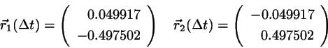
Since we have
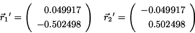
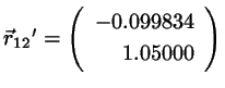
. Insert this in the correction
formula 4.8-4.9 to find
(4.16)
which is identical to the exact values.
Thermostats / Nosé-Hoover method:
In a nonequilibrium process work must be invested which systematically
heats up the system. In lab experiments a thermostat takes care of this;
in simulations the problem of thermostating is non-trivial.
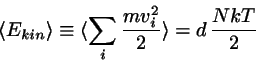
The temperature of a molecular dynamics sample is not an input parameter
to be manipulated at will; rather, it is a quantity to be ``measured'' in terms of an average of the kinetic energy of the particles,
( dimension).
Suggestions as to how one can maintain a desired
temperature in a dynamical simulation range from repeatedly rescaling
all velocities (``brute force thermostat'') to adding a suitable
stochastic force acting on the molecules.
Such recipes are unphysical and introduce an artificial trait of
irreversibility and/or indeterminacy into the microscopic dynamics.
A interesting deterministic method of thermostating a simulation
sample was introduced by Shuichi Nosé and William Hoover.
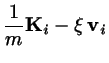
Under very mild conditions the following augmented equations of motion
will lead to a correct sampling of the canonical phase space at a given
temperature :
The coupling parameter describes the inertia of the thermostat.
The generalized viscosity is temporally varying and may assume
negative values as well.
For systems of many degrees of freedom (particles) this is sufficient
to produce a pseudo-canonical sequence of states.
For low-dimensional systems it may be necessary to use two NH thermostats
in tandem [MARTYNA 92].
 etc. The only constraint is
 and
and
![$\displaystyle \frac{2}{Q}\left[ E_{kin}-3NkT_{0}/2 \right]$](img317.png)