5.2 Pair Correlation Function

Let

$$a(\mbox{$\bf r$};\mbox{$\bf\Gamma$}_{c}) = \sum_{i}\delta(\mbox{$\bf r$}_{i}-\mbox{$\bf r$})$$

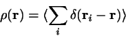
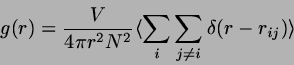
An average of this quantity represents the relative frequency, or probability densitiy of some particle being situated near $\mbox{$\bf r$}$. In other words, $\langle a(\mbox{$\bf r$})\rangle=\rho(\mbox{$\bf r$})$ is simply the mean fluid density at position $\mbox{$\bf r$}$:

$$\rho(\mbox{$\bf r$})=\langle \sum_{i}\delta(\mbox{$\bf r$}_{i}-\mbox{$\bf r$})\rangle$$

In a fluid we usually have $\rho(\mbox{$\bf r$})=const$; only in the presence of external fields or near surfaces $\rho(\mbox{$\bf r$})$ varies in a non-trivial manner.

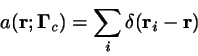
Let us proceed to the ``pair correlation function'' (PCF)

$$g(r)=\frac{V}{4\pi r^{2}N^{2}} \langle\sum_{i}\sum_{j\neq i} \delta (r-r_{ij}) \rangle$$ (5.1)

This is the conditional probability density of finding a particle at $\mbox{$\bf r$}$, given that there is a particle at the coordinate origin. Thus $g(r)$ provides a measure of local spatial ordering in a fluid.

To determine $g(r)$, proceed like this:

• Divide the range of $r$-values (at most $[0;L/2]$, where $L$ is the side length of the basic cell) into $50-200$ intervals of length $\Delta r$.
• A given configuration $\{ \mbox{$\bf r$}_{1},\dots\mbox{$\bf r$}_{N}\}$ is scanned to determine, for each pair $(i,j)$, a ``distance channel''number
  
  $$k=\mbox{int}\left( \frac{r_{ij}}{\Delta r}\right)$$
  
  

• In a histogram table $g(k)$ the corresponding value is then incremented by $1$. This procedure is repeated every, say, $50$ MD steps (or $50N$ MC steps).
• At the end of the simulation run the histogram is normalized according to 5.1.

The typical shape of the PCF at liquid densities is depicted in Fig. 5.1.

Figure 5.1: Pair correlation function of the Lennard-Jones liquid

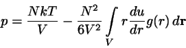
Significance of $g(r)$ in fluid physics:

• The average of any quantity that depends on the pair potential $u(r)$ may be expressed as an integral over $g(r)$.
  Example: pressure (see also 1.2)
  
  $$p=\frac{NkT}{V}-\frac{N^{2}}{6V^{2}}\int\limits_{V}r\frac{du}{dr}g(r) d\mbox{$\bf r$}$$
  
  
  
  
  
• Theory: analytical approximations to $g(r)$ for a given pair potential $u(r)$.[KOHLER 72],[HANSEN 86]
• Experiment: the Fourier transform of $g(r)$, the ``scattering law''
  
  $$S(k)=1+ \frac{N}{V}\int\limits_{V}[g(r)-1] e^{\textstyle i \mbox{$\bf k$}\cdot \mbox{$\bf r$}} d\mbox{$\bf r$}$$
  
  
  is just the relative intensity of neutron or X-ray scattering at a scattering angle $\theta$ with
  
  $$k\equiv\frac{4\pi}{\lambda}\sin \frac{\theta}{2}$$
  
  

PROJECT MD/MC (LENNARD-JONES): Augment your Lennard-Jones MD (or MC) program by a routine that computes the pair correlation function $g(r)$ according to 5.2; remember to apply the nearest image convention when computing the pair distances. As the subroutine ENERGY already contains a loop over all particle pairs $(i,j)$, it is best to increment the $g(r)$ histogram within that loop.

Plot the PCF and see whether it resembles the one given in Figure 5.1.