Consider two parallel lines of finite lengths $L_{1,2} = 2h_{1,2}$ containing a homogeneous
density of square well centers. Let $\vec{r}_{1,2}$ and be the position
of the two line centers, and write $\vec{r}_{12}$ for the vector between the centers.
By assumption both direction vectors are $\vec{e}_{1,2}= \vec{e} \equiv (0,0,1)$;
therefore, taking advantage of symmetry, we will now use cylindrical coordinates,
writing the relative vector between particle centers as
$\vec{r}_{12} = \left( \rho, z \right)$.
For convenience we may always assume that $z \geq 0$; otherwise we
let $z \rightarrow -z$, with no change of potential. We also require
$h_{2} \geq h_{1}$, with no loss of generality.
Let $\lambda, \, \mu$ be the parameters giving the positions of
the interacting points along $1$ and $2$. The squared distance between
any two such points is given by
$r^{2}(\lambda,\mu)= \rho^{2}+ \left( z + \mu - \lambda \right)^{2}$.
The total interaction energy between the two lines is then
with $u_{SW}(r)= \infty $ if $r < s_{1}$, $= - \varepsilon $
if $s_{1} < r < s_{2}$, and $=0$ for $r > s_{2}$. Typically,
$s_{1}=1.0$ and $s_{2}=1.5 - 2.0$.
In the $(\lambda, \mu )$ plane the integration region is
represented by a rectangle $R$ with sides $L_{1,2}$ around
$(0,0)$. However, the integrand is non-zero, and constant,
only for $ r^{2}(\lambda, \mu ) < s_{2}^{2}$.
In other words, the integral gives the area shared by the rectangle
$R$ and a region $E$ between the two parallels described by
$\mu^{\pm}(\lambda) = (\lambda - z) \pm \sqrt{s_{2}^{2}-\rho^{2}}$.
The potential between two SWL particles is given by
the area of the overlap region between the rectangle
$R:
\{ \lambda \, \epsilon \, [\mp h_{1} ] , \,
\mu \, \epsilon \, [\mp h_{2} ] \}$
and the region $E$ between the lines
$\mu^{\pm}(\lambda) = (\lambda - z) \pm \sqrt{s_{2}^{2}-\rho^{2}}$.
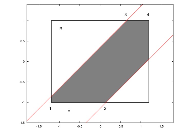
Figure 1: Square Well Lines, parallel: The potential is given by the overlap area
of the rectangle and the region between the red lines defined by
$\mu(\lambda) = $ $(\lambda - z) \pm $ $\sqrt{s_{2}^{2}-\rho^{2}}$.
The figure refers to a pair
with lengths $L_{1}=2.4$, $L_{2}=2.$, and $s_{2}=1.5$; the $z$ displacement is
$z = 0.4$, and the perpendicular distance $\rho=1.3$. Points $1$ and $2$ are
defined thus: find the intersection of the horizontal line
$ \mu = \mu_{l} = -L_{2}/2 $ with
the upper
and lower red line, respectively; if that intersection is outside the lower
rectangle side, move to the nearest end of that side.
Points $3$ and $4$ are defined similarly but referring to the upper rectangle border,
$ \mu = \mu_{u} = L_{2}/2 $.
The task of computing the shaded area of Fig. 1 may seem trivial, but we have to
define a procedure that comprises all possible configurations of the interacting
sticks, and thus of $R$ and $E$. The following box presents this procedure in
a self-contained formulation.
Computing $u(1,2)$ for two unequal, parallel SW Lines:
Let $\vec{r}_{1,2}$ be given, as well
as the lengths $L_{1,2} \equiv 2h_{1,2}$ and the square well limits
$s_{1}$ and $s_{2}$; the particles are assumed to point in the $z$
direction. The particle index $2$ is reserved for the longer stick,
if any. To calculate $u(1,2)$ proceed as follows:
Make sure that $z \; (= z_{12}) \geq 0 $; otherwise let
$z \rightarrow -z$.
Make sure that the SW particles have no overlap, i.e. contain
no points with a mutual distance below
$s_{1}$: if $\rho^{2} > s_{1}^{2}$,
there can be no overlap; else we have to discern the cases
(a) $ z \leq h_{1}+h_{2}$ (overlap) and (b) $ z > h_{1}+h_{2}$
which leads to overlap if
$ \rho^{2}+(z-(h1+h2))^{2} \leq s_{1}^{2} $.
Using $ s_{2} $ in place of $ s_{1} $
we can ascertain if there is any non-zero interaction at all.
From now on we
assume that there is an interaction but no hard overlap.
Determine points $1$ and $2$ by computing the intersection points
of the lower rectangle side $\mu = \mu_{l} \equiv -h_{2}$
with the upper/lower red lines
(i. e. interaction range limits) given by
$\mu^{\pm}(\lambda) = (\lambda - z) \pm$ $ \sqrt{s_{2}^{2}-\rho^{2}}$;
the desired points are either these intersections
or the nearest endpoints of the lower rectangle side. The same relations
are used to determine points $3$ and $4$ which refer to the intersection
between the upper rectangle border
$\mu = \mu_{u} \equiv h_{2}$
and the red lines:
$\lambda_{1,2} =
min ( h_{1}, \, max (-h_{1}, z-h_{2}
\mp \sqrt{s_{2}^{2}-\rho^{2}}\, ) \, )
\;\;\;\;\;\;\;\;\;\;(2.1)
$
$\lambda_{3,4} =
min ( h_{1}, \, max (-h_{1}, z+h_{2}
\mp \sqrt{s_{2}^{2}-\rho^{2}}\, ) \, )
\;\;\;\;\;\;\;\;\;\;(2.2)
$
Compute the overlap area $A$ (grey in Fig. 1) according to
for given values of the $z$ displacement.
Equs. 2-5, while useful
for the calculation of specific
pair energies, do not contain the explicit forms of $\lambda_{i}(\rho)$
and are therefore not suited to a formal integration over $\rho$.
Here we derive an alternative expression for $u(\rho,z)$, making the
$\rho$-dependence explicit.
The terms $I_{0}$, $I_{12}^{-}$ and $I_{34}^{+}$ depend on pairwise combinations
of $\lambda_{1-4}$, namely (1,4), (1,2), and (3,4). The functional forms
of $\lambda_{i}(\rho)$ change between different regions of $\rho$.
For example, $\lambda_{1}(\rho) = -h_{1}$ (constant) for all configurations
in which $z-h_{2}-\sqrt{s_{2}^{2}-\rho^{2}} \leq -h_{1}$, or
$\rho^{2} \leq s_{2}^{2}-(z-h_{2}+h_{1})^{2}$.
In Figure 1 this corresponds to those situations in which the upper red line
crosses the base of the rectangle left of its left boundary - as
in the case sketched there.
On the other hand, the form $\lambda_{1}(\rho) = $
$z-h_{2}-\sqrt{s_{2}^{2}-\rho^{2}}\,$
will hold when the intersection occurs within the base line boundaries,
$\pm h_{1}$. Quantifying these considerations for all $\lambda_{i}(\rho)$
we may easily identify the various $\rho$ intervals. First we introduce the
following parameters:
For given values of $z \geq 0$, $h_{1}$ and $h_{2} \geq h_{1}$ we have
$f_{1} \geq e_{1}$ and $f_{0} \leq e_{0}$. The limits of hard overlap
and of outer interaction range are
$\rho_{min}^{2} \equiv max \left(\,0, \, s_{1}^{2}-e_{1}^{2} \, \right) $ and
$\rho_{max}^{2} \equiv max \left(\,0, \, s_{2}^{2}-e_{1}^{2} \, \right) $.
Within that relevant interaction region we define the following interval
boundaries:
Obviously, $\rho_{1} \leq \rho_{2}$, $\rho_{4} \leq \rho_{3}$, and
$\rho_{5} \leq \rho_{6}$. Using these definitions we find the following scheme:
Case
$\lambda_{1}(\rho)$
$ \rho$ interval
1A
$-h_{1}$
$
\left[\,\rho_{min}, \, \rho_{1} \, \right]
$
1B
$z-h_{2}-\sqrt{s_{2}^{2}-\rho^{2}}$
$
\left[\, \rho_{1}, \, \rho_{max} \,\right]
$
1C
$+h_{1}$
$ - $
Case
$\lambda_{2}(\rho)$
$ \rho $ interval
2A
$-h_{1}$
$
\left[\, \rho_{3}, \,\rho_{max}\,\right]
$
2B
$z-h_{2}+\sqrt{s_{2}^{2}-\rho^{2}}$
$
\left[\, \rho_{4},\, \rho_{3}\,\right]
$
2C
$+h_{1}$
$
\left[\,\rho_{min}, \, \rho_{4}\,\right]
$
Case
$\lambda_{3}(\rho)$
$ \rho $ interval
3A
$-h_{1}$
$
\left[\,\rho_{min}, \,\rho_{5} \,\right]
$
3B
$z+h_{2}-\sqrt{s_{2}^{2}-\rho^{2}}$
$
\left[\, \rho_{5},\, \rho_{6}\,\right]
$
3C
$+h_{1}$
$
\left[\, \rho_{6}, \,\rho_{max}\,\right]
$
Case
$\lambda_{4}(\rho)$
$ \rho $ interval
4A
$-h_{1}$
$
-
$
4B
$z+h_{2}+\sqrt{s_{2}^{2}-\rho^{2}}$
$
-
$
4C
$+h_{1}$
$
\left[\,\rho_{min}, \,\rho_{max}\,\right]
$
Table 1: For given $z$ the functions
$\lambda_{i}(\rho)$ retain their form over the given intervals. The
notation is obvious: 1A means that $\lambda_{1}'$ is left of the
base line of the rectangle, 1B...on the base line, 1C...right of the base line.
The expressions 4.1-4.3 for $I_{0}$ etc.
contain pairs of $\lambda_{i}$. Obviously, the $\rho$ intervals in which
these combinations have a certain functional form are the intersections of
the respective pair of intervals in the foregoing list.
Here follows a complete listing of all non-trivial combinations of $\lambda$
and regions of $\rho$, together with the functional form of $I_{0}$,
$I_{12}^{-}$ and $I_{34}$, as well as their respective integral functions;
for convenience we use the name $t \equiv \sqrt{s_{2}^{2}-\rho^{2}}$ for
that frequently occuring term:
Table 2: For given $z$ the relevant $\rho$ intervals are listed (second
column).
Within these intervals, some of which may be of zero width, the functions
$I_{0}(\rho)$ etc. and their integral
functions are listed (third and fourth rows.)
* Note: the expressions in column 3 may in principle be used as
alternative formulae to equs. 2-5
to compute individual pair energies at specific ($z, \rho$); in that
case only non-zero intervals must be considered.
Here is a short resume:
Area integral of the potential for parallel SWL sticks
We want to calculate the integral
$
J(z) \equiv 2 \pi \int d\rho' \, \rho \, u(\rho'; z)
$
where
$
u(\rho; z) = (- \varepsilon/L_{1}L_{2}) ( I_{0} + I_{12}^{-} - I_{34}^{+} )
$
as in eq. 3.
Since the functional form of $u(\rho; z)$ varies in different $\rho$
intervals we have to identify these intervals before we can formally
integrate:
() Determine the parameters
$ \rho_{min,max} $ and $ \rho_{1-6} $
(eqs. 8.1-8.6);
() insert these as limits
in the expressions for $J_{0} \equiv 2 \pi \int d\rho' \, \rho' I_{0}(\rho')$ etc.
as in Table 2;
() these terms are summed over all intervals (rows) and
combined to give $J(z)=J_{0}+J_{12}^{-}-J_{34}^{+}$.
A Java Applet is
here
A Fortran code is deposited
here