With his ``Kinetic Theory of Gases'' Boltzmann undertook to explain
the properties of dilute gases by analysing the elementary collision
processes between pairs of molecules.
The evolution of the distribution density in space,
, is described by
Boltzmann's transport equation. A thorough treatment of this
beautiful achievement is beyond the scope of our discussion.
But we may sketch the basic ideas used in its derivation.
If there were no collisions at all, the swarm of particles
in space would flow according to
(2.1)
where denotes an eventual external force acting on particles at
point
. The time derivative of is therefore,
in the collisionless case,
(2.2)
where
(2.3)
and
(2.4)
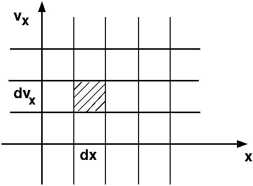
To gather the meaning of equation 2.2 for free flow, consider
the collisionless, free flow of gas particles through
a thin pipe: there is no force (i. e. no change of velocities),
and -space has only two dimensions, and (see Figure
2.2).
A very simple mu-space
At time a differential ``volume element'' at contains,
on the average,
particles. The temporal
change of is then given by
(2.5)
To see this, count the particles entering during the time span
from the left (assuming ,
and those leaving towards the right,
. The local change per unit time is then
(2.6)
(2.7)
(2.8)
(2.9)
(2.10)
(2.11)
The relation
is then easily generalized to the case of a non-vanishing force,
(2.12)
(this would engender an additional vertical flow in the figure),
and to six instead of two dimensions (see equ. 2.2).
All this is for collisionless flow only.
In order to account for collisions a term
is added on the right hand side:
(2.13)
The essential step then is to find an explicit expression
for
. Boltzmann solved this problem
under the simplifying assumptions that
- only binary collisions need be considered (dilute gas);
- the influence of container walls may be neglected;
- the influence of the external force (if any) on the rate
of collisions is negligible;
- velocity and position of a molecule are uncorrelated
(assumption of molecular chaos).
The effect of the binary collisions is expressed in terms of a
``differential scattering cross section''
which describes the probability density for a certain
change of velocities,
(2.14)
( thus denotes the relative orientation of the vectors
and
).
The function
depends on the intermolecular potential
and may be either calculated or measured.
Under all these assumptions, and by a linear expansion of the left
hand side of equ. 2.1 with respect to time, the
Boltzmann equation takes on the following form:
(2.15)
where
,
etc.
This integrodifferential equation describes, under the given assumptions,
the spatio-temporal behaviour of a dilute gas. Given some initial
density
in -space the solution
function
tells us how this density changes over
time. Since has up to six arguments it is difficult to visualize; but
there are certain moments of which represent measurable averages
such as the local particle density in 3D space, whose temporal change
can thus be computed.
Chapman and Enskog developed a general procedure for the approximate
solution of Boltzmann's equation. For certain simple model systems such as
hard spheres their method produces predictions for
(or its moments) which
may be tested in computer simulations. Another more modern approach to
the numerical solution of the transport equation is the
``Lattice Boltzmann'' method in which the continuous variables
and are restricted to a set of discrete values; the
time change of these values is then described by a modified transport
equation which lends itself to fast computation.
The initial distribution density
may be
of arbitrary shape. To consider a simple example, we may have
all molecules assembled in the left half of a container - think
of a removable shutter - and at time make the rest of the
volume accessible to the gas particles:
(2.16)
where
is the (Maxwell-Boltzmann) distribution
density of particle velocities, and
denotes
the Heaviside function. The subsequent expansion of the gas
into the entire accessible volume, and thus the approach to the stationary
final state (= equilibrium state) in which the particles are evenly
distributed over the volume may be seen in the solution
of Boltzmann's equation.
Thus the greatest importance of this equation is its ability to describe
also non-equilibrium processes.
The Equilibrium distribution
is that solution of Boltzmann's equation which is
stationary, meaning that
(2.17)
It is also the limiting distribution for long times,
.
It may be shown that this equilibrium distribution is given by
(2.18)
where and are the local density and temperature,
respectively.
If there are no external forces such as gravity or electrostatic interactions
we have
. In case the temperature is also
independent of position, and if the gas as a whole is not moving
(), then
, with
 Applet BM:
Start
Applet BM:
Start
![$\textstyle \parbox{360pt}{
\mbox{}\\
{\bf Simulation: The power of Boltzmann's...
...tion densities in r-space and in v-space
\\
\vspace{2ex}
{\small [Code: BM]}
}$](img488.png)