1.3 Fundamentals of Statistics

By statistics we denote the investigation of regularities in apparently non-deterministic processes. An important basic quantity in this context is the ``relative frequency'' of an ``event''. Let us consider a repeatable experiment - say, the throwing of a die - which in each instance leads to one of several possible results $e$ - say, $e \equiv number of points = 4$. Now repeat this experiment $n$ times under equal conditions and register the number of cases in which the specific result $e$ occurs; call this number $f_{n}(e)$. The relative frequency of $e$ is then defined as $r(e)$ $\equiv f_{n}(e)/n$.

Following R. von Mises we denote as the ``probability '' of an event $e$ the expected value of the relative frequency in the limit of infinitely many experiments:

$${\cal P}(e) \equiv \lim_{n \rightarrow \infty} \frac{f_{n}(e)}{n}$$ (1.24)

EXAMPLE: Game die; 100-1000 trials; $e \equiv \{no. of points = 6\}$, or $e \equiv \{no. of points$ $\leq 3\}$.

Now, this definition does not seem very helpful. It implies that we have already done some experiments to determine the relative frequency, and it tells us no more than that we should expect more or less the same relative frequencies when we go on repeating the trials. What we want, however, is a recipe for the prediction of ${\cal P}(e)$.

To obtain such a recipe we have to reduce the event $e$ to so-called ``elementary events'' $\epsilon$ that obey the postulate of equal a priori probability. Since the probability of any particular one among $K$ possible elementary events is just ${\cal P}(\epsilon_{i}) = 1/K$, we may then derive the probability of a compound event by applying the rules

$${\cal P}(e = \epsilon_{i} \; or \; \epsilon_{j}) = {\cal P}(\epsilon_{i}) +{\cal P}(\epsilon_{j})$$ (1.25)

$${\cal P}(e = \epsilon_{i} \; and \; \epsilon_{j}) = {\cal P}(\epsilon_{i}) \cdot{\cal P}(\epsilon_{j})$$ (1.26)

Thus the predictive calculation of probabilities reduces to the counting of the possible elementary events that make up the event in question.

EXAMPLE: The result $\epsilon_{6} \equiv \{no. of points =6\}$ is one among $6$ mutually exclusive elementary events with equal a priory probabilities ($=1/6$). The compound event $e \equiv \{ no. of points \leq 3\}$ consists of the elementary events $\epsilon_{i} =\{1, 2 or 3 \}$; its probability is thus ${\cal P}(1\vee 2\vee 3)= 1/6 + 1/6 + 1/6 = 1/2$.

How might this apply to statistical mechanics? - Let us assume that we have $N$ equivalent mechanical systems with possible states $s_{1}, s_{2}, \dots s_{K}$. A relevant question is then: what is the probability of a situation in which

$$e \equiv \{ k_{1} systems are in state s_{1}, \; k_{2} systems in state s_{2}, etc. \}$$ (1.27)

EXAMPLE: $N=60$ dice are thrown (or one die $60$ times!). What is the probability that $10$ dice each have numbers of points $1, 2, \dots 6$? What, in contrast, is the probability that all dice show a ``one''?

The same example, but with more obviously physical content:
Let $N=60$ gas atoms be contained in a volume $V$, which we imagine to be divided into $6$ equal partial volumes. What is the probability that at any given time we find $k_{i}=10$ particles in each subvolume? And how probable is the particle distribution $(60,0,0,0,0,0$)? (Answer: see below under the heading ``multinomial distribution''.)

We can generally assume that both the number $N$ of systems and the number $K$ of accessible states are very large - in the so-called ``thermodynamic limit'' they are actually taken to approach infinity. This gives rise to certain mathematical simplifications.

Before advancing into the field of physical applications we will review the fundamental concepts and truths of statistics and probability theory, focussing on events that take place in number space, either $\cal R$ (real numbers) or $\cal N$ (natural numbers).


DISTRIBUTION FUNCTION
Let $x$ be a real random variate in the region $(a,b)$. The distribution function

$$P(x_{0}) \equiv {\cal P} \{x < x_{0}\}$$ (1.28)

is defined as the probability that some $x$ is smaller than the given value $x_{0}$. The function $P(x)$ is monotonically increasing and has $P(a)=0$ and $P(b)=1$. The distribution function is dimensionless: $\left[ P(x) \right] = 1$.

The most simple example is the equidistribution for which

$$P(x_{0})= \frac{x_{0}-a}{b-a}$$ (1.29)

Another important example, with $a=- \infty$, $b=\infty$, is the normal distribution

$$P(x_{0})= \frac{1}{\sqrt{2\pi}} \int_{-\infty}^{x_{0}} dx e^{-x^{2}/2}$$ (1.30)

and its generalization, the Gaussian distribution

$$P(x_{0})= \frac{1}{\sqrt{2\pi \sigma^{2}}} \int_{-\infty}^{x_{0}} dx e^{-(x- \langle x \rangle)^{2}/2 \sigma^{2}}$$ (1.31)

where the parameters $\langle x \rangle$ and $\sigma^{2}$ define an ensemble of functions.


DISTRIBUTION DENSITY
The distribution or probability density $p(x)$ is defined by

$$p(x_{0}) dx \equiv {\cal P} \{ x \in [x_{0}, x_{0}+dx] \} \equiv dP(x_{0})$$ (1.32)

In other words, $p(x)$ is just the differential quotient of the distribution function:

$$p(x)= \frac{dP(x)}{dx} , \;\;\; {\rm i.e.} \;\; P(x_{0})= \int_{a}^{x_{0}} p(x) dx$$ (1.33)

$p(x)$ has a dimension; it is the reciprocal of the dimension of its argument $x$:

$$\left[ p(x) \right] = \frac{1}{[x]}$$ (1.34)

For the equidistribution we have

$$p(x)= 1/(b-a),$$ (1.35)

and for the normal distribution

$$p(x)= \frac{1}{\sqrt{2\pi}} e^{-x^{2}/2}.$$ (1.36)

If $x$ is limited to discrete values $x_{\alpha}$ with a step $\Delta x_{\alpha} \equiv x_{\alpha+1}-x_{\alpha}$ one often writes

$$p_{\alpha} \equiv p(x_{\alpha}) \Delta x_{\alpha}$$ (1.37)

for the probability of the event $x=x_{\alpha}$. This $p_{\alpha}$ is by definition dimensionless, although it is related to the distribution density $p(x)$ for continuous arguments. The definition 1.37 includes the special case that $x$ is restricted to integer values $k$; in that case $\Delta x_{\alpha} = 1$.


MOMENTS OF A DENSITY
By this we denote the quantities

$$\langle x^{n} \rangle \equiv \int_{a}^{b} x^{n} p(x) dx \... ...; case, \;\;\;} \equiv \sum_{\alpha} p_{\alpha} x_{\alpha}^{n}$$ (1.38)

The first moment $\langle x \rangle$ is also called the expectation value or mean value of the distribution density $p(x)$, and the second moment $\langle x^{2} \rangle$ is related to the variance and the standard deviation: variance $\sigma^{2} = \langle x^{2} \rangle - \langle x \rangle ^{2}$ (standard deviation $\sigma$ = square root of variance).

EXAMPLES:
.) For an equidistribution $\epsilon [0, 1]$ we have $\langle x \rangle = 1/2$, $\langle x^{2} \rangle =1/3$ and $\sigma^{2}= 1/12$.
.) For the normal distribution we find $\langle x \rangle =0$ and $\langle x^{2} \rangle =\sigma^{2}=1$.

SOME IMPORTANT DISTRIBUTIONS

$\bullet$ Equidistribution: Its great significance stems from the fact that this distribution is central both to statistical mechanics and to practical numerics. In the theory of statistical-mechanical systems, one of the fundamental assumptions is that all states of a system that have the same energy are equally probable (axiom of equal a priori probability). And in numerical computing the generation of homogeneously distributed pseudo-random numbers is relatively easy; to obtain differently distributed random variates one usually ``processes'' such primary equidistributed numbers.

$\bullet$ Gauss distribution: This distribution pops up everywhere in the quantifying sciences. The reason for its ubiquity is the ``central value theorem'': Every random variate that can be expressed as a sum of arbitrarily distributed random variates will in the limit of many summation terms be Gauss distributed. For example, when we have a complex measuring procedure in which a number of individual errors (or uncertainties) add up to a total error, then this error will be nearly Gauss distributed, regardless of how the individual contributions may be distributed. In addition, several other physically relevant distributions, such as the binomial and multinomial densities (see below), approach the Gauss distribution under certain - quite common - circumstances.

Figure 1.9: Equidistribution and normal distribution functions $P$ and densities $p$

$\bullet$ Binomial distribution: This discrete distribution describes the probability that in $n$ independent trials an event that has a single trial probability $p$ will occur exactly $k$ times:

$$p_{k}^{n} \equiv {\cal P} \{ k \;\; {\rm times\; e \; in \; n \; trials}\}$$

$$= {n \choose k} p^{k} (1-p)^{n-k}$$ (1.39)

For the first two moments of the binomial distribution we have $\langle k \rangle =np$ (not necessarily integer) and $\sigma^{2}= np(1-p)$ (i.e. $\langle k^{2} \rangle - \langle k \rangle ^{2}$).

Figure 1.10: Binomial distribution density $p_{k}^{n}$

APPLICATION: Fluctuation processes in statistical systems are often described in terms of of the binomial distribution. For example, consider a particle freely roaming a volume $V$. The probability to find it at some given time in a certain partial volume $V_{1}$ is $p(V_{1})=V_{1}/V$. Considering now $N$ independent particles in $V$, the probability of finding just $N_{1}$ of them in $V_{1}$ is given by

$$p_{N_{1}}^{N} = {N \choose N_{1}} (V_{1}/V)^{N_{1}} (1-V_{1}/V)^{N-N_{1}}$$ (1.40)

The average number of particles in $V_{1}$ and its standard deviation are

$$\langle N_{1} \rangle = N V_{1}/V \;\; {\rm and} \; \; \sigm... ...\sqrt{(\Delta N_{1})^{2}} = \sqrt{N (V_{1} / V) (1-V_{1}/V)}.$$ (1.41)

Note that for $Np \approx 1$ we have for the variance $\sigma^{2} \approx \sigma \approx \langle N_{1} \rangle \approx 1$, meaning that the population fluctuations in $V_{1}$ are then of the same order of magnitude (namely, $1$) as the mean number of particles itself.

For large $n$ such that $np » 1$ the binomial distribution approaches a Gauss distribution with mean $np$ and variance $\sigma^{2}=npq$ (theorem of Moivre-Laplace):

$$p_{k}^{n} \Rightarrow p_{G}(k)=\frac{1}{\sqrt{2 \pi npq}} \exp{[-(k-np)^{2}/2npq]}$$ (1.42)

with $q \equiv 1-p$.

If $n \rightarrow \infty$ and $p \rightarrow 0$ such that their product $np \equiv \lambda$ remains finite, the density 1.39 approaches

$$p_{n}(k) = \frac{\lambda^{k}}{k!} e^{-\lambda}$$ (1.43)

which goes by the name of Poisson distribution.

An important element in the success story of statistical mechanics is the fact that with increasing $n$ the sharpness of the distribution 1.39 or 1.42 becomes very large. The relative width of the maximum, i. e. $\sigma/\langle k \rangle$, decreases as $1/\sqrt{n}$. For $n=10^{4}$ the width of the peak is no more than $1 \%$ of $\langle k \rangle$, and for ``molar'' orders of particle numbers $n \approx 10^{24}$ the relative width $\sigma/\langle k \rangle$ is already $\approx 10^{-12}$. Thus the density approaches a ``delta distribution''. This, however, renders the calculation of averages particularly simple:

$$\langle f(k) \rangle = \sum_{k} p_{k}^{n}f(k) \rightarrow f(\langle k \rangle )$$ (1.44)

or

$$\langle f(k) \rangle \approx \int dk \delta (k-\langle k \rangle) f(k) = f(\langle k \rangle )$$ (1.45)

$\bullet$ Multinomial distribution: This is a generalization of the binomial distribution to more than 2 possible results of a single trial. Let $e_{1},e_{2},\dots ,e_{K}$ be the (mutally exclusive) possible results of an experiment; their probabilities in a single trial are $p_{1},p_{2},\dots, p_{K}$, with $\sum_{i}^{K}p_{i}=1$. Now do the experiment $n$ times; then

$$p_{n}(k_{1},k_{2},\dots, k_{K}) = \frac{n!}{k_{1}! k_{2}! \d... ...s p_{K}^{k_{K}} \;\;\;(with \;\;k_{1}+k_{2}+ \dots +k_{K} = n)$$ (1.46)

is the probability to have the event $e_{1}$ just $k_{1}$ times, $e_{2}$ accordingly $k_{2}$ times, etc.

We get an idea of the significance of this distribution in statistical physics if we interpret the the $K$ possible events as ``states'' that may be taken on by the $n$ particles of a system (or, in another context, by the $n$ systems in an ensemble of many-particle systems). The above formula then tells us the probability to find $k_{1}$ among the $n$ particles in state $e_{1}$, etc.

EXAMPLE: A die is cast $60$ times. The probability to find each number of points just $10$ times is

$$p_{60}(10,10,10,10,10,10) = \frac{60!}{(10!)^{6}} \left( \frac{1}{6}\right)^{60} = 7.457 \cdot 10^{-5} .$$ (1.47)

To compare, the probabilities of two other cases: $p_{60}(10,$ $10,10,10,9,11)$ $= 6.778 \cdot 10^{-5}$, $p_{60}(15,15,15,5,5,5)$ $= 4.406 \cdot 10^{-8}$. Finally, for the quite improbable case $(60,0,0,0,0,0)$ we have $p_{60}=2.046 \cdot 10^{-47}$

Due to its large number of variables ($K$) we cannot give a graph of the multinomial distribution. However, it is easy to derive the following two important properties:

Approach to a multivariate Gauss distribution: just as the binomial distribution approaches, for large $n$, a Gauss distribution, the multinomial density approaches an appropriately generalized - ``multivariate'' - Gauss distribution.

Increasing sharpness: if $n$ and $k_{1}\dots k_{K}$ become very large (multiparticle systems; or ensembles of $n \rightarrow \infty$ elements), the function $p_{n}(k_{1},k_{2},\dots, k_{K})$ $\equiv p_{n} (\vec{k})$ has an extremely sharp maximum for a certain partitioning $\vec{k}^{*}\equiv \{ k_{1}^{*}, k_{2}^{*}, \dots, k_{K}^{*}\}$, namely $\{ k_{i}^{*}$ $=n p_{i}; i=1, \dots, K \}$. This particular partitioning of the particles to the various possible states is then ``almost always'' realized, and all other allotments (or distributions) occur very rarely and may safely be neglected.

This is the basis of the method of the most probable distribution which is used with great success in several areas of statistical physics.[2.2]

STIRLING'S FORMULA
For large values of $m$ the evaluation of the factorial $m!$ is difficult. A handy approximation is Stirling's formula

$$m! \approx \sqrt{2 \pi m} (m/e)^{m}$$ (1.48)

EXAMPLE: $m=69$ (Near most pocket calculators' limit): $69! = 1.7112 \cdot 10^{98}$; $\sqrt{2 \pi \cdot 69} (69/e)^{69} = 1.7092 \cdot 10^{98}$.

The same name Stirling's formula is often used for the logarithm of the factorial:

$$\ln m! \approx m (\ln m -1) + \ln \sqrt{2 \pi m} \approx m (\ln m -1)$$ (1.49)

(The term $\ln \sqrt{2 \pi m}$ may usually be neglected in comparison to $m (\ln m -1)$.)

EXAMPLE 1: $\ln 69! = 226.1905$; $69(\ln 69 - 1) + \ln \sqrt{2 \pi \cdot 69} = 223.1533 + 3.0360 = 226.1893$.

EXAMPLE 2: The die is cast again, but now there are $120$ trials. When asked to produce $120!$ most pocket calculators will cancel their cooperation. So we apply Stirling's approximation:
The probability of throwing each number of points just $20$ times is

$$p_{120}(20,\dots,20) = \frac{120!}{(20!)^{6}} \left( \frac{1... ...ht)^{20} \frac{1}{20!} \right]^{6} = 1.350 \cdot 10^{-5} ,$$ (1.50)

and the probability of the partitioning $(20,20,20,20,19,21)$ is $1.285 \cdot 10^{-5}$.

STATISTICAL (IN)DEPENDENCE
Two random variates $x_{1}, x_{2}$ are statistically mutually independent (uncorrelated) if the distribution density of the compound probability (i.e. the probability for the joint occurence of $x_{1}$ and $x_{2}$) equals the product of the individual densities:

$$p(x_{1},x_{2}) = p(x_{1}) p(x_{2}) .$$ (1.51)

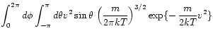
EXAMPLE: In a fluid or gas the distribution density for a single component of the particle velocity is given by (Maxwell-Boltzmann)

$$p(v_{\alpha}) = \sqrt{\frac{m}{2 \pi kT}} \exp\{-\frac{m v_{\alpha}^{2}}{2 k T} \}, \;\; \alpha = x,y,z$$ (1.52)

The degrees of freedom $\alpha = x,y,z$ are statistically independent; therefore the compound probability is given by

$$p(\vec{v}) \equiv p(v_{x},v_{y},v_{z}) = p(v_{x}) p(v_{y}) p... ...{3/2} \exp\{-\frac{m}{2 kT} (v_{x}^{2}+v_{y}^{2}+v_{z}^{2}) \}$$ (1.53)

By conditional distribution density we denote the quantity

$$p(x_{2} \vert x_{1}) \equiv \frac{p(x_{1},x_{2})}{p(x_{1})}$$ (1.54)

(For uncorrelated $x_{1}, x_{2}$ we have $p(x_{2} \vert x_{1}) =$ $p(x_{2})$).

The density of a marginal distribution describes the density of one of the variables regardless of the specific value of the other one, meaning that we integrate the joint density over all possible values of the second variable:

$$p(x_{2}) \equiv \int_{a_{1}}^{b_{1}} p(x_{1},x_{2}) dx_{1}$$ (1.55)

TRANSFORMATION OF DISTRIBUTION DENSITIES
From 1.32 we can immediately conclude how the density $p(x)$ will transform if we substitute the variable $x$. Given some bijective mapping $y=f(x); \; x=f^{-1}(y)$ the conservation of probability requires

$$\vert dP(y) \vert = \vert dP(x)\vert$$ (1.56)

(The absolute value appears because we have not required $f(x)$ to be an increasing function.) This leads to

$$\vert p(y) dy \vert = \vert p(x) dx\vert$$ (1.57)

or

$$p(y)= p(x) \left\vert \frac{dx}{dy}\right\vert = p[f^{-1}(y)] \left\vert \frac{df^{-1}(y)}{dy} \right\vert$$ (1.58)

Incidentally, this relation is true for any kind of density, such as mass or spectral densities, and not only for distribution densities.

EXAMPLE 1: A particle of mass $m$ moving in one dimension is assumed to have any velocity in the range $\pm v_{0}$ with equal probability; so we have $p(v)=1/2v_{0}$. The distribution density for the kinetic energy is then given by (see Figure 1.11)

$$p(E) = 2 p(v) \left\vert \frac{dv}{dE} \right\vert = \frac{1}{2 \sqrt{E_{0}}} \frac{1}{\sqrt{E}}$$ (1.59)

in the limits $0 .. E_{0}$, where $E_{0}=mv_{0}^{2}/2$. (The factor $2$ in front of $p(v)$ comes from the ambiguity of the mapping $v \leftrightarrow E$).

Figure 1.11: Transformation of the distribution density (see Example 1)

EXAMPLE 2: An object is found with equal probability at any point along a circular periphery; so we have $p(\phi) = 1/2 \pi$ for $\phi \epsilon [ 0, 2 \pi ]$. Introducing cartesian coordinates $x = r \cos \phi$, $y = r \sin \phi$ we find for the distribution density of the coordinate $x$, with $x \epsilon [\pm r]$, that

$$p(x) = p(\phi) \left\vert \frac{d \phi}{dx} \right\vert = \frac{1}{\pi} \frac{1}{\sqrt{r^{2}-x^{2}}}$$ (1.60)

(see Figure 1.12)

Problems equivalent to these examples:
a) A homogeneously blackened glass cylinder - or a semitransparent drinking straw - held sideways against a light source: absorption as a function of the distance from the axis?
b) Distribution of the $x$-velocity of a particle that can move randomly in two dimension, keeping its kinetic energy constant.

$\Rightarrow \;$ Simulation 1.6: Stadium Billiard. Distribution of the velocity component $v_{x}$. [Code: Stadium]

c) Distribution of the velocity of any of two particles arbitrarily moving in one dimension, keeping only the sum of their kinetic energies constant.

Figure 1.12: Transformation of the distribution density (see Example 2)

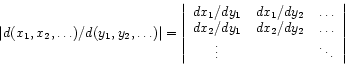
For the joint probability density of several variables the transformation formula is a direct generalization of 1.58, viz.

$$p(\vec{y})= p(\vec{x}) \left\vert \frac{d\vec{x}}{d\vec{y}}\right\vert$$ (1.61)

Here we write $\left\vert d\vec{x}/d\vec{y}\right\vert$ for the functional determinant (or Jacobian) of the mapping $\vec{x} = \vec{x}(\vec{y})$,

$$\left\vert d(x_{1},x_{2}, \dots)/d(y_{1},y_{2},\dots)\right\... ...}/dy_{2} & \dots \\ \vdots & & \ddots \end{array}\right\vert$$ (1.62)

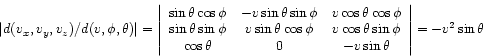
EXAMPLE 3: Again, let $\vec{v} \equiv \{v_{x},v_{y},v_{z}\}$, and $p(\vec{v})$ as in equ. 1.53. Now we write $\vec{w}$ $\equiv \{ v, \phi, \theta \}$, with

$$v_{x} = v \sin \theta \cos \phi, \;\; v_{y} = v \sin \theta \sin \phi, \;\; v_{z} = v \cos \theta .$$ (1.63)

The Jacobian of the mapping $\vec{v} = \vec{v}(\vec{w})$ is

$$\left\vert d(v_{x},v_{y},v_{z})/d(v,\phi,\theta)\right\vert=... ... & -v \sin \theta \end{array}\right\vert = - v^{2} \sin \theta$$ (1.64)

Therefore we have for the density of the modulus of the particle velocity

$$p(v) \equiv \int_{0}^{2 \pi} d \phi \int_{- \pi}^{\pi} d \theta v^{2} \sin \theta \left( \frac{m}{2 \pi kT} \right)^{3/2} \exp\{- \frac{m}{2 kT} v^{2} \}$$ (1.65)

$$= 4 \pi \left( \frac{m}{2 \pi kT} \right)^{3/2} v^{2} \exp\{- \frac{m}{2 kT} v^{2} \}$$ (1.66)