4 Evaluation of Simulation Experiments
Subsections
4.1 Thermodynamic Averages
At time $t$, combine the position vectors of the
$N$ atoms into a vector
$\Gamma_{c} \equiv \{ r_{1} \dots r_{N} \}$
The set of all possible such vectors spans the
$3N$-dimensional "configuration space" $\Gamma_{c}$.
Let $a(\Gamma_{c})$ be a property of the $N$-body system, depending on
the positions of all particles, i.e. of the microstate
$ \Gamma_{c}$. The thermodynamic average of $a$ is given by
$
\langle a \rangle = \int_{\Gamma_{c}} a(\Gamma_{c})
\,p(\Gamma_{c})\, d \Gamma_{c}
$
where $p(\Gamma_{c})$ is the probability density
at the configuration space point $\Gamma_{c}$.
Examples:
- Internal energy:
$
U=NkT+\frac{1}{2} \langle \, \sum_{i} \sum_{j \neq i}
u(r_{ij}) \, \rangle
$
- Pressure:
$
p=\frac{NkT}{V} - \frac{1}{6V} \langle \, \sum_{i} \sum_{j \neq i}
r_{ij} \left. \frac{du}{dr} \right|_{r_{ij}} \rangle
$
Problem: the probability density $p(\Gamma_{c})$
is known only up to an indetermined normalizing factor.
Thus, $p_{can}(\Gamma_{c})$ $\propto exp[-E(\Gamma_{c})/kT]$,
but the normalizing denominator $Q$ (the Configurational Partition
Function) in
$
1 = \int p(\Gamma_{c})\, d \Gamma_{c} \equiv \frac{1}{Q}
\int e^{\textstyle -E(\Gamma_{c})/kT} \, d \Gamma_{c}
$
is not known.
Spin systems:
Basic model of ferromagnetic solids:
atoms are fixed on the vertices of a lattice. Their
dipole vectors (spins) may have varying directions: either
up/down (Ising model) or any direction (Heisenberg model).
Microscopic configuration $ \Gamma_{c}$: given by the
$N$ spins on the lattice.
Example:
Two-dimensional square Ising lattice; only the four nearest spins
contribute to the energy of spin $\sigma_{i}$
($= \pm 1$). (Three dimensions: six nearest neighbors).
The total energy is
$
E=-\frac{A}{2}\sum_{i=1}^{N} \sum_{j(i)=1}^{4\; or \;6} \sigma_{i}
\sigma_{j(i)}
$
($A$ ... coupling constant).
$\Longrightarrow$ Magnetic polarization
$
M \equiv \sum_{i=1}^{N} \sigma_{i}
$
may be determined as a function of temperature.
If a magnetic field $H$ is applied, the additional potential energy is
$E_{H}=-H \sum_{i} \sigma_{i}$.
More averages:
In addition to basic thermodynamic observables such as
internal energy and pressure many more details about the structure
and the dynamics of statistical-mechanical systems may be accessed.
Below we will consider two such quantities, the
pair correlation function $g(r)$
and the velocity autocorrelation function $C(t)$.
PROJECT MD/MC (LENNARD-JONES):
In your Lennard-Jones MD and MC programs, include a procedure to
calculate averages of the total potential energy and the virial
as defined by
$
W\equiv\sum_{i}\vec{K}_{i}\cdot \vec{r}_{i} = -\frac{1}{2}\sum_{i}\sum_{j}
\vec{K}_{ij}\cdot \vec{r}_{ij}
$
From these compute the internal energy and the pressure.
Compare with results from literature, e.g. [
MCDONALD 74,
VERLET 67].
Allow for deviations in the
$5-10 \%$ range, as we have
omitted a correction for the finite sample size ("cutoff correction").
4.2 Pair Correlation Function
Let
$
a( r;\Gamma_{c}) = \sum_{i}\delta( r_{i}- r)
$
An average of this quantity represents the relative frequency,
or probability densitiy of some
particle being situated near
$ r$. In other words,
$\langle a( r)\rangle=\rho( r)$ is simply the mean
fluid density at position $ r$:
$
\rho( r)=\langle \sum_{i}\delta( r_{i}- r)\rangle
$
In a fluid we usually have
$\rho( r)=const$; only in the presence
of external fields or near surfaces $\rho( r)$
varies in a non-trivial manner.
Let us proceed to the "pair correlation function" (PCF)
$
g(r)=\frac{\textstyle V}{\textstyle 4\pi r^{2}N^{2}}
\langle\sum_{i}\sum_{j\neq i} \delta (r-r_{ij}) \rangle
$
This is the
conditional probability density of finding a particle at
$ r$,
given that there is a particle at the coordinate origin.
Thus
$g(r)$
provides a measure of local spatial ordering in a fluid.
To determine
$g(r)$, proceed like this:
- Divide the range of $r$
-values (at most $[0;L/2]$, where
$L$ is the side length of the basic cell) into
$50-200$ intervals of length $\Delta r$.
- A given configuration $\{ r_{1},\dots r_{N}\}$
is scanned to
determine, for each pair
$(i,j)$, a "distance channel" number
$
k=\mbox{int}\left( \frac{\textstyle r_{ij}}{\textstyle \Delta r}\right)
$
- In a histogram table
$g(k)$
the corresponding value is then incremented by
$1$. This procedure is repeated every, say,
$50$ MD steps (or $50N$
MC steps).
- At the end of the simulation run the histogram is normalized according to
5.1.
The typical shape of the PCF at liquid densities is depicted in
Fig. 5.1.
Figure 5.1:
Pair correlation function of the Lennard-Jones liquid
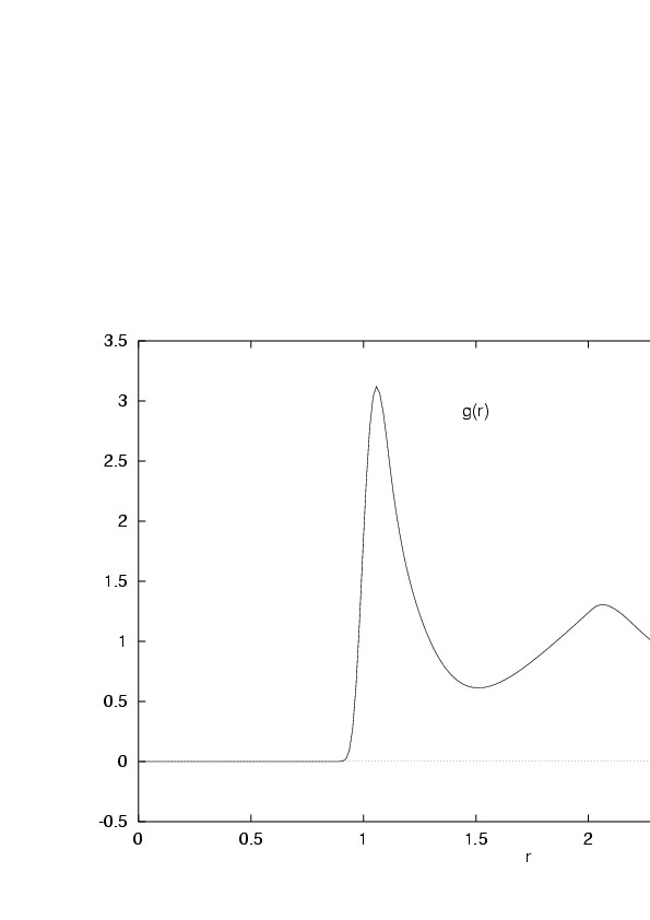
|
Significance of $g(r)$ in fluid physics:
- The average of any quantity that depends on the pair
potential $u(r)$ may be expressed as an integral over $g(r)$.
Example: pressure (see also 1.2)
$
p=\frac{\textstyle NkT}{\textstyle V}-\frac{\textstyle N^{2}}{\textstyle 6V^{2}}
\int\limits_{V}r\frac{\textstyle du}{\textstyle dr} g(r) dr
$
- Theory: analytical approximations to
$g(r)$ for a given pair potential $u(r)$.
[KOHLER 72],
[HANSEN 86]
- Experiment: the Fourier transform of $g(r)$, the
"scattering law"
$
S(k)=1+ \frac{\textstyle N}{\textstyle V}\int\limits_{V}[g(r)-1]
e^{\textstyle i k\cdot r} d r
$
is just the relative intensity of neutron or X-ray scattering at
a scattering angle $\theta$ with
$
k\equiv\frac{\textstyle 4\pi}{\textstyle \lambda}
\sin \frac{\textstyle \theta}{\textstyle 2}
$
PROJECT MD/MC (LENNARD-JONES):
Augment your Lennard-Jones MD (or MC) program by a routine that
computes the pair correlation function
$g(r)$ according to 5.2; remember to apply the
nearest image convention
when computing the pair distances.
As the subroutine ENERGY already contains a loop over all
particle pairs $(i,j)$, it is best to increment the
$g(r)$ histogram within that loop.
Plot the PCF and see whether it resembles the one given in
Figure 5.1.
4.3 Autocorrelation Functions
An elementary example of temporal correlations of the form
$
C_{a}(t) \equiv \langle a(0) a(t) \rangle
$
is the velocity autocorrelation in fluids
$
C(t)\equiv \langle v_{i}(0)\cdot v_{i}(t)\rangle
$
Simple kinetic theory, which takes into account only binary
collisions, predicts
$C(t)\propto e^{-\lambda t}$. At fluid densities
a different behavior is to be expected. Nevertheless the first results on
$C(t)$obtained by
Alder [ALDER 67]
provided some surprises.
It turned out that at intermediate fluid densities and long times
$C(t) \propto t^{-3/2}$ instead of showing an exponential decay.
This has profound consequences. The diffusion constant $D$
of a liquid is given by
$
D=\frac{1}{3}\int\limits_{0}^{\infty}C(t) dt
$
Due to the long time tail of $C(t)$ the simulation result for
$D$ is about $30$ percent larger than its kinetic estimate.
The reason for the long time tail in $C(t)$
was later explained as a
collective dynamical effect: part of the momentum of a particle
is stored in a microscopic vortex that dies off very
slowly.[DORFMAN 72]
Figure 5.2:
Velocity autocorrelation function of the Lennard-Jones fluid
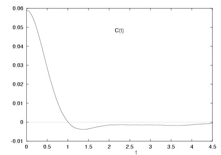
|
Procedure for calculating autocorrelation functions
$$ $<a(0) a(t)>$:
- At regular intervals of
$20-100$ time steps, mark starting values
$\{a(t_{0,m}),m=1,\dots M\}$.
Since in the further process only the
preceding $M \approx 10-20$
starting values are required, it is best to store
them in registers that are cyclically overwritten.
- At each time $t_{n}$, compute the $M$ products
$
z_{m}=a(t_{n})\cdot a(t_{0,m}),\;\;\;m=1,\dots M
$
and relate them to the (discrete) time displacements
$\Delta t_{m}\equiv t_{n}-t_{0,m}$
$\Delta t_{m}\equiv t_{n}-t_{0,m}$
; a particular
$\Delta t_{m}$
defines
a channel number
$
k=\Delta t_{m}/\Delta t
$
indicating the particular histogram channel to be incremented by
$z_{m}$.
To simplify the final normalization it is recommended to count the number
of times each channel $k$ is incremented.
EXERCISE:
Run your MD program for $2000$
time steps and store the velocity vector
of a certain particle (say, no. 1) at each time step. Write and test a
program that evaluates the autocorrelation function of this vector.
PROJECT MD (LENNARD-JONES):
Using the experience gathered in the above exercise, write a procedure
that computes the velocity ACF, averaged over all particles, during
an MD simulation run.
Plot the ACF and see whether it resembles the one given in
Figure 5.2.
vesely
2005-10-10