I am doing MC (Np) of N equal triblock particles consisting of an axial
spherocylinder and a central sphere. The spherocylinder width
is $D$, the cylinder length is $L$; the width of the central sphere
is called $\sigma$.
For a quick orientation I have done some simulations with $N=108$.
Taking $D$ as the unit of length, I chose $L=9$ and varied $\sigma$,
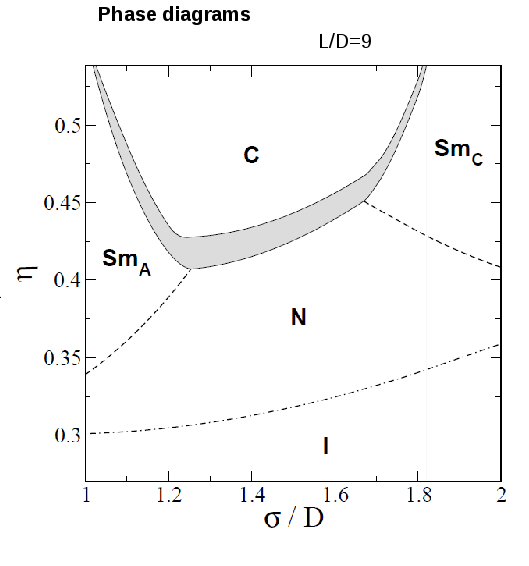
so as to compare with Szabi's PPT slide 19 (Figure 1).
From your theoretical results I expect that for $\sigma =1.0$
a smectic phase should occur for $\eta \, \epsilon \, (0.35, 0.55)$. This
phase should shrink and disappear on increasing $\sigma \rightarrow 1.2$.
Let us see whether we can reproduce this behaviour by MC simulation.
Density modes and smectic phases
Let
$
\rho(\vec{k}) \equiv \frac{\textstyle 1}{\textstyle V}\sum_{j=1}^{N}
e^{\textstyle -i\vec{k}\cdot \vec{r}_{j}}
$
with $V = c_{x}^{2}\,c_{z}$ (square prism box)
denote the Fourier component of the particle density corresponding to a
Fourier vector $\vec{k}$.
Writing $\rho(\vec{k}) = \rho'(\vec{k}) - i \, \rho''(\vec{k})$ with
$
\rho'(\vec{k}) = \frac{\textstyle 1}{\textstyle V}\sum_{j=1}^{N}
\cos \left( \vec{k}\cdot \vec{r}_{j} \right)
$
and
$
\rho''(\vec{k}) = \frac{\textstyle 1}{\textstyle V}\sum_{j=1}^{N}
\sin \left( \vec{k}\cdot \vec{r}_{j} \right)
$
the normalized structure factor
$S(\vec{k}) \equiv \left[ \rho'^{2} + \rho''^{2} \right] /
(N/V)^{2} $ may vary between
$0$ and $1$. Any inhomogeneity
in the system will be indicated by enhanced values of
certain structure factors. If $S(\vec{k})$ is small, the liquid is more or
less homogeneous along the respective $\vec{k}$. Smectic layering
announces itself by a high value of some $S(\vec{k})$, where $\vec{k}$
is the layer normal. If $\vec{k}$ points along the $z$ axis we have a
smectic A phase, otherwise smectic C.
Figure 1: Theoretical prediction for the phase boundaries of parallel
Martini Olives with $L/D=9$ and $(\sigma/D) \, \epsilon \, (1.0, 2.0)$.
(From Sz. Varga, PPT document "Triblock Summary", 2010; slide 19.)
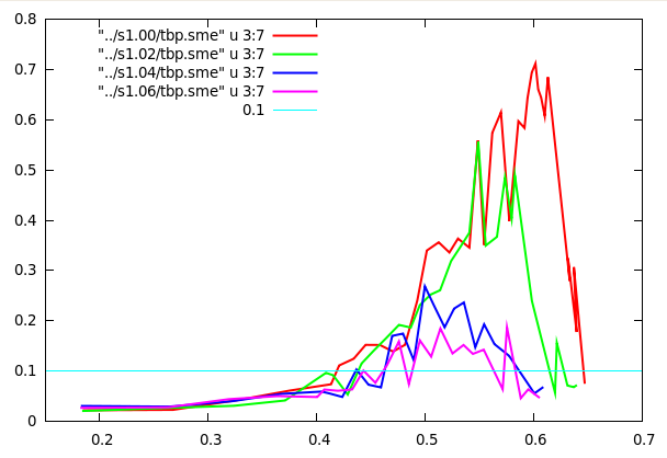
Figure 2 shows the results of preliminary runs with 108 MO particles.
Abscissa: $\eta$; ordinate: $S(\vec{k}_{m})$, the largest Fourier
amplitude of the density correlation. The strongest mode, and thus the
associated vector $\vec{k}_{m}$, may change along a curve
as long as $S$ is insignificantly low ($< 0.1$); but for higher
values of $S$ it is always $\vec{k}=(0,0,3)$ for the given system
size.
Let us define the onset of smectic ordering, somewhat arbitrarily,
by the smectic amplitude rising above $S=0.1$. According to
this simple rule we see that only for $\sigma=1.0-1.06$ smectic
ordering may be observed. At $\sigma=1.06$ the amplitude barely
crosses $0.1$. Comparing this to Szabi's slide 19, the range of smecticity
ends sooner. Also, the $\eta$ values are higher:
$\eta_{sme} \, \epsilon \, (0.44, \, 0.59)$ for $\sigma=1.04$
and $1.06$, $\eta_{sme} \, \epsilon \, (0.42, \, 0.62)$ for $\sigma=1.02$,
and $\eta_{sme} \, \epsilon \, (0.41,\, 0.64)$ for $\sigma=1.0$. The latter
case compares well with the Bolhuis-Frenkel paper of 1996. (BF use
$\rho* = \rho/\rho_{cp}$ instead of $\eta$,
and the appropriate interval from their Figure 2 is
$\rho* \, \epsilon \, (0.5,\, 0.7)$ which in our case is equivalent to
$\eta \, \epsilon \, (0.45, \, 0.63)$.)
I hope that the jumpiness of the curves will decrease when I go to
higher particle numbers.
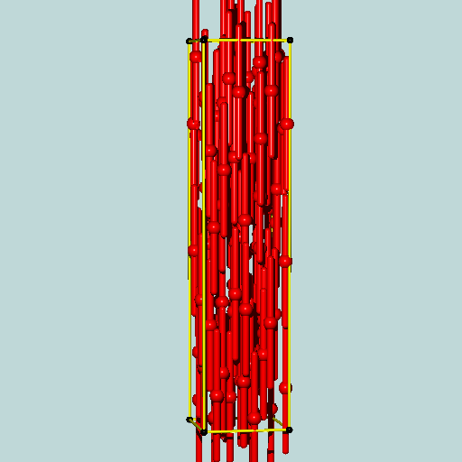
At the right end of Szabi's plot we have the SmC phase. In the simulation
this phase is hard to attain, since the particles get locked in a
metastable low density configuration (Figure 3). I am still groping for
a way to nudge them into a more dense arrangement without forcing the
issue. But maybe I should start out with a SmC phase and
decompress it. Will play around some more.
FV Dec 7, 2010
Figure 2: Simulation results for $N=108$.
Figure 3: Non-ergodic situation in MC of Triblock particles
with $D=\sigma/2$.
Jan 7, 2011:
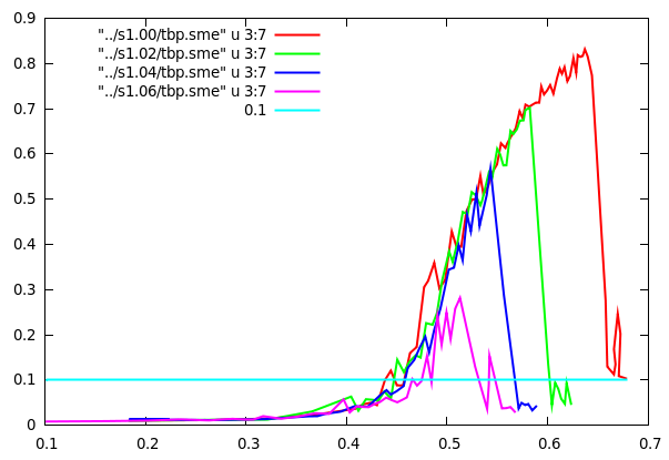
Figure 4 shows the results of a set of MC runs with $N=256$. Again, the central
sphere width was $\sigma=$ $1.00$, $1.02$, $1.04$, and $1.06$ ($L=9$, $d=1$.)
Compared to the exploratory runs shown in Figure 2 the curves are much smoother,
with a more well-defined upper limit for $\eta$. The intervals of smecticity
are now
$\eta_{sme} \, \epsilon \, (0.45, \, 0.66)$ for $\sigma=1.00$,
$\eta_{sme} \, \epsilon \, (0.45, \, 0.61)$ for $\sigma=1.02$,
$\eta_{sme} \, \epsilon \, (0.46, \, 0.57)$ for $\sigma=1.04$, and
$\eta_{sme} \, \epsilon \, (0.48, \, 0.53)$ for $\sigma=1.06$.
I have no news yet about $\sigma > 1.8$.
FV Jan 7, 2011
Figure 4: Simulation results for $N=256$.
Feb 15, 2011:
First, let me display the January 7 results as a table (cf. Figure 4):
$\sigma$
$\eta$ range
$S_{max}$
$d_{0}$
1.00
0.44-0.66
0.83
11.5-9.9
1.02
0.45-0.60
0.70
11.2-10.2
1.04
0.46-0.57
0.57
11.0-10.3
1.06
0.47-0.53
0.28
10.9-10.5
Table 1: Simulation results for small central
spheres (see Figs. 1 and 4). (The numbers
differ a bit from the Jan 7 note, as I take
them directly from the Fortran output, not
from the graph.)
The value of $d_{0}$ should be taken with a grain of salt. The
periodic simulation cell can accomodate only an integer number
(in our case, four) of smectic layers. If necessary, the layer
distances will adjust slightly to fit into the cell; if the
discrepancy is too large, the smectic
structure will break down. In our results a slightly shorter
period $d_{0}$ as compared with theory is noticeable, but the
smecticity is never in danger.
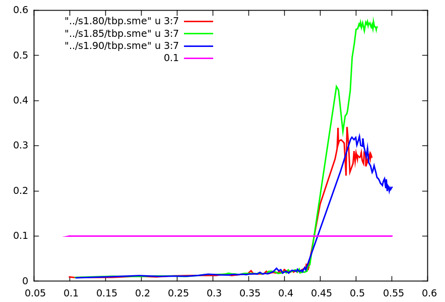
And here, at last, are my results for $\sigma \geq 1.8$.
In Figure 5, the largest Fourier amplitudes for central sphere diameters
$\sigma = 1.80$, $1.85$, and $1.90$ are displayed. It is obvious that
near $\eta = 0.45$ a smectic-C phase appears. However, the preferred
$k$ vector is still changing with further compression. For example,
in the system with $\sigma=1.80$ the integer components of
$\vec{k}$ are $(5/-2/4)$ in the range $\eta = 0.44-0.49$, then
switch to $(-3/-3/4)$. The smectic period changes accordingly,
from $d_{0}=2.1$ to $2.6$. The complete table of results is here:
$\sigma$
$\eta$
$k_{xyz}$
$S_{max}$
$d_{0}$
1.80
0.44-0.49
5/-2/4
0.34
2.1
1.80
0.49-...
-3/-3/4
0.29
2.6
1.85
0.45-0.48
0/-5/4
0.43
2.3
1.85
0.48-0.49
*
*
*
1.85
0.49-...
3/3/4
0.57
2.6
1.90
0.45-...
-5/1/4
0.32
2.2
Table 2: Smectic-C phases for large central spheres
from MC simulation (see Fig. 5). The starlets denote
fluctuating $k$ vectors and wave lengths.
It is clear that the transition from SmC to columnar cannot be
attained in the simulation - the densities are too high.
FV Feb 15, 2011
Note added Feb-22: Table 2a is the same as Table 2 but includes
the smectic-C angles:
$\sigma$
$\eta$
$k_{xyz}$
$\Psi$
$S_{max}$
$d_{0}$
1.80
0.44-0.49
5/-2/4
76.7
0.34
2.1
1.80
0.49-...
-3/-3/4
73.3
0.29
2.6
1.85
0.45-0.48
0/-5/4
75.4
0.43
2.3
1.85
0.48-0.49
*
*
*
*
1.85
0.49-...
3/3/4
73.0
0.57
2.6
1.90
0.45-...
-5/1/4
75.5
0.32
2.2
Table 2a: Smectic-C phases for large central spheres (same as
Table 2 but including smectic-C angles.)
Figure 5: Results for $\sigma = 1.80-1.90$ ($N=256$)
Mar 17, 2011:
New table 2: It seems that the cell shapes I used in the first two runs,
$c_{z}/c_{x} \approx. 3.1$ and $ \approx 6.6$, led to metastable states with
a non-optimal smectic-C structure. This can be seen from the rather low
$S_{max}$ values for $ \sigma=1.8$ and $1.9$.
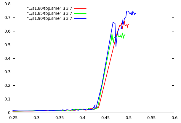
Based on this experience I did a new set of compression runs, using a very
different shape $c_{z}/c_{x}=4.5$. It turns out that now the results are very
consistent, and the attainable values of $S_{max}$ are much higher for all
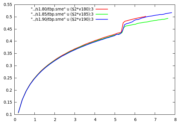
three $\sigma $. Also, a plot of $\eta$ vs pressure shows definite jumps
at the transition points.
Actually, we should use the locus of the steep density increase as the
indication of the nematic-smectic-C transition, which is much more
satisfactory and "physical" than the arbitrary criterion $S_{max}=0.1$.
I have done this in the following new version of table 2. Also, I have
included the $\Psi$ angle.
$\sigma$
$\Delta \eta$
$k_{xyz}$
$\Psi$
$S_{max}$
$d_{0}$
1.80
0.44-0.48
-5/ 2/4
80.6
0.67
1.9
1.85
0.43-0.46
-3/ 5/4
81.3
0.58
1.8
1.90
0.43-0.47
-5/ 2/4
80.6
0.75
1.9
Table 2 (new): Smectic-C phases for large central spheres from
MC simulation (see Fig. 5). $\Delta \eta$ ... density difference btw.
nematic and smectic-C phase; $k_{xyz}$...integer components of the
smectic vector. Note that the k vector is also determined by
the shape of the simulation cell; in our case, $c_{z}=4.5\,c_{x}$,
therefore $\vec{k}=(2 \pi/c_{x}) (k_{x}, k_{y}, k_{z}/4.5)$.
Figure 6: New results for $\sigma = 1.80-1.90$ ($N=256$).
Much higher $S_{max}$; obviously, the smectic C phase was
reached.
Figure 7: $\eta$ vs. $P v_{0}$, where $v_{0}$ is the
particle volume.