| |
|
THE SHAPE OF THINGS
Morphology of hard bodies and excluded volumes
CECAM Workshop "Simulations of hard bodies"
Lyon, April 2007
Sponsored by: Cecam, Simbioma, ESF, COST
Lectio nec urbe nec Lugduno recitata
|
| |
|
|
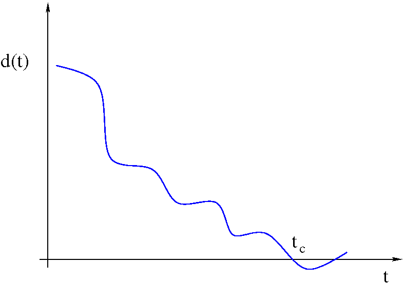
Figure 1: Surface-surface distance $d$ as function of time
|
We seek an economical (quick) method to determine the first
zero-line
crossing of $d(t)$. The function $d(t)$ depends on the shapes $r_{s}$
and orientations $\Omega(t)$ of the bodies.
Alternative:
Let $r_{c}(\Omega_{1},\Omega_{2})$ denote the contact (center-center)
distance at the given orientations; then the function
$\tilde{d}(t) \equiv r(t)-r_{c}(t)$ has the same zeros as $d(t)$.
However, $r_{c}$ may be computed in advance, before the actual simulation.
Here is what we need:
-
Ways to describe the shape of a particle, either implicitly via
a constraint equation, or explicitly by some
expression for the surface points, $\vec{r}_{s}(\vec{\alpha})$ or
$r_{s}(\vec{\alpha})$, where $\vec{\alpha}$
denotes some internal coordinates (usually angles.)
-
Ways to describe the "shape" of $r_{c}(\Omega_{1},\Omega_{2})$,
the contact (center-center) distance at the given orientations, which is
a characteristic of the mutually excluded volume.
$(\Omega_{1},\Omega_{2})$ may amount to 2,3, or 5 arguments.
-
Ways to describe the evolution of $\Omega$ in time. There are
beautiful papyri
on this in the literature.
|
|
|
I
|
Reminder:
One particle has no meaning; two make a substance. The only relevant probe
to determine the shape of a particle is another particle.
The problem $r_{s} \longrightarrow r_{c}$ is always solvable, if not
always uniquely. The inverse problem $r_{c} \longrightarrow r_{s}$ is
overdetermined.
The "Protean" HGO and HLJL models are actually defined
via their pair contact distance; they have no individual shape.
But:
-
We like to visualize individual particles
-
Often a simple geometric shape is desirable as input to theory.
Therefore: let us discuss $r_{s}$ for a while, keeping in mind
that it is mostly just assumed and may be taken with a grain of salt.
And for the treatment of the actual collision event we will need some $r_{s}$
after all: point of contact; transfer of momenta etc.
|
|
| II |
-
Constraint equations
-
$r_{s}$ or $r_{s}^{2}$ expanded in basis functions
-
$\vec{r}_{s}$ expanded in basis functions (EFA, Elliptical
Fourier Analysis)
-
Constraint equations
-
Prime example: Ellipse/Ellipsoid
$
\sigma(\vec{r},C) \equiv \vec{r}^{T} \cdot C \cdot \vec{r} - 1 = 0
$
may be understood as a constraint eqn.; useful e.g. for finding
the normal vector at some boundary point $R(\vec{r})$:
$\vec{n} = \lambda \nabla_{R} \sigma$.
-
Spherocylinder
Again, the requirement of equal (a) point-line distance from
axis (for cylinder wall) or (b) point-point distance
from end points (for caps) may be seen as a constraint eqn.,
$
\sigma \equiv \left | \vec{r} - \vec{p} \right| - R = 0,
\;\;\;\;$ if $ \vec{r}$ is athwart of the axis;
$
\sigma \equiv \left| \vec{r}-\vec{r}_{a,b} \right| -R = 0
\;\;\;\;$ else $\qquad \qquad \qquad \qquad $
where $\vec{p}$ is a point on the axis in a normal plane through
$\vec{r}$, and $\vec{r}_{a,b}$ are the end points of the axis.
-
Others:
Superellipsoids / Spheroellipsoids (F. V.) /
Fused spheres / etc.
may be described this way.
To find the surface-surface distance, we may start from the
constraint eqns. and apply one of the available strategies:
() Perram-Wertheim (for ellipsoids)
() Newton-Raphson à la De Michele
()
"Gliders" method (F. V.):
-
two virtual particles
constrained to remain on their respective ellipsoid surfaces but
attracting each other by a harmonic force;
- apply SHAKE to let them
find the closest postions (proxy points)
Pretty quick; probably
equivalent to Newton-Raphson; likely to be
restricted to convex or at least starlike particles.
-
Series expansion of
rs or rs2
Usually done in circular or spherical harmonics;
for symmetric tops a Chebysheff polynomial expansion along the $z$ axis
is also possible, see
Smectic demixing: Koda theory
-
Ellipse / Circular Harmonics:
Let the long axis $a$ point up ($y$) and count polar angle
$\theta$ from $y$ axis; then
$
r_{s}(\theta) =
\frac{\textstyle a b}{\textstyle \sqrt{a^{2} \sin^{2} \theta + b^{2} \cos^{2} \theta}}
$
may be expanded as Fourier series in $\theta$:
$r_{s}(\theta)=\sum_{k=0}^{K} a_{k} \cos k\theta$.
-
Ellipsoid, symmetric or asymmetric / Spherical Harmonics:
$r_{s}$ as above; may be expanded in
spherical harmonics. Since for symmetric ellipsoids the
azimuthal angle $\phi$ is irrelevant, Legendre polynomials
$P_{k}(\theta)$ suffice:
$
r_{s}(\theta) = \sum \limits_{k=0}^{K} c_{k} P_{k} (\theta)
\;\;\;\;{\rm with} \;\;\;\;
c_{k} = \frac{1}{..}\int d cos\theta \; r_{s}(\theta) P_{k} (\theta)
$
otherwise, use $Y_{k}^{m}$:
$
r_{s}(\theta, \phi) =
\sum \limits_{k=0}^{K} \sum \limits_{m=-k}^{k} c_{km} Y_{k}^{m} (\theta, \phi)
\;\;\;\;{\rm with} \;\;\;\;
c_{km} = \frac{1}{..}\int d cos\theta \int d\phi \;
r_{s}(\theta) Y_{k}^{m} (\theta,\phi)
$
where $1/..$ denotes the appropriate normalization.
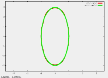
As a specific example, here are an ellipse and a superellipse with $n=6$
together with their Fourier representations.
|
|
|
|
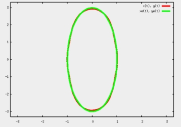
Figure 2: Ellipse/Superellipse, original vs. Fourier reproduction
(8 terms)
|
The task of finding the surface-surface distance and the related
contact distance $r_{c}(\Omega_{1},\Omega_{,2})$ is painful:
-
Choose plausible $\theta$ $\phi$ on both contours;
-
compute $r_{s}^{(1,2)}(\theta,\phi)$ from the Fourier series;
insert these $r_{s}$ in $x'=r_{s} \sin \theta \cos \phi$
etc. and transform $\vec{r}'=\{x',y',z'\}$ to lab coordinates
$\vec{r}=\{x,y,z\}$;
-
improve $\vec{r}^{(1,2)}$ by Newton-Raphson or similar such
that $\left| \vec{r}^{(2)} -\vec{r}^{(1)} \right|$ is
minimized.
-
Elliptical Fourier Analysis (EFA)
Starting from the parametric representation of an ellipse,
$
\begin{eqnarray}
x(t)&=& x_{0}+ a_{1,1} \cos \frac{2\pi t}{T}
+ a_{1,2} \sin \frac{2\pi t}{T}
\\
y(t)&=&
y_{0}+ a_{2,1} \cos \frac{2\pi t}{T}
+ a_{2,2} \sin \frac{2\pi t}{T}
\end{eqnarray}
$
where $T$ is the perimeter of the ellipse,
we generalize these expressions, writing
$
\begin{eqnarray}
x(t)&=&x_{0}+\sum \limits_{k=1}^{K}
\left[ a_{1,2k-1} \cos \frac{2\pi k t}{T}
+ a_{1,2k} \sin \frac{2\pi k t}{T} \right]
\\
y(t)&=&y_{0}+\sum \limits_{k=1}^{K}
\left[ a_{2,2k-1} \cos \frac{2\pi k t}{T}
+ a_{2,2k} \sin \frac{2\pi k t}{T} \right]
\end{eqnarray}
$
or
$
\vec{r}_{s} = \vec{r}_{0} + A \cdot \vec{w}
$
with $A$ the matrix of coefficients, and
$
\vec{w} \equiv \left\{ w_{2k-1}, w_{2k} ; \, k=1, ..\right\}^{T}
= \left\{ \cos (2 k \pi t/T), \sin(2 k \pi t/T) ; \, k=1, ..\right\}^{T}
$
Note that the argument $2 \pi k t / T$, although by
definition an angle, is not identical to the polar angle
in the ellipse.
Inversion: Given a table of points
$\{x_{i},y_{i}, i=1,N \}$ on an arbitrary closed contour the
elements of $A$ may be computed according to
$
\begin{eqnarray}
a_{1,2k-1}&=&
\frac{\textstyle T}{\textstyle 2k^{2}\pi^{2} }
\sum \limits_{i=1}^{N} \frac{\textstyle \Delta x_{i}}{\textstyle \Delta t_{i} }
\left[
\cos \frac{\textstyle 2 \pi k t_{i} }{\textstyle T }
-\cos \frac{\textstyle 2 \pi k t_{i-1} }{\textstyle T }
\right]
\\
a_{1,2k}&=&
\frac{\textstyle T}{\textstyle 2k^{2}\pi^{2} }
\sum \limits_{i=1}^{N} \frac{\textstyle \Delta x_{i}}{\textstyle \Delta t_{i} }
\left[
\sin \frac{\textstyle 2 \pi k t_{i} }{\textstyle T }
-\sin \frac{\textstyle 2 \pi k t_{i-1} }{\textstyle T }
\right]
\end{eqnarray}
$
et mut. mut.
|
|
|
|
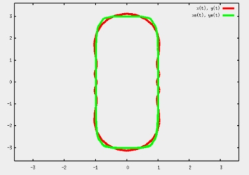
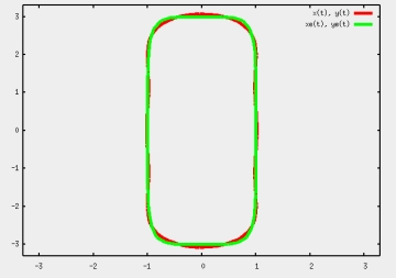
Figure 3: Ellipse/Superellipse, original vs. EFA
(5 harmonics)
|
Finding the surface-surface distance and the related
contact distance $r_{c}(\Omega_{1},\Omega_{,2})$:
"Gliders" method is simplified, as we need not
enforce the constraint (" stay on the contour!");
the matrix $A$ defines the contour.
Here is the procedure:
|
|
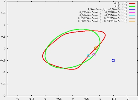
Figure 4: Gliding along a weird contour (red). The blue external
point attracts a glider confined to the red outline. The estimated
starting point is drawn in light blue.
|
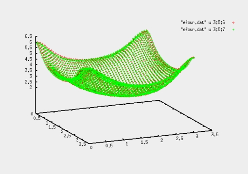
Extension to 3D? $\Longrightarrow$ Use $Y_{k}^{m}$ in place
of cos/sin.
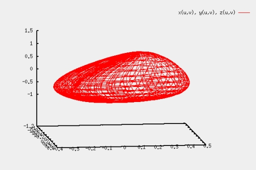
Just playing around with a few low order terms produces this:
|
|
Figure 5: A weird 3D surface
|
No inversion formulae in the literature, but may be
worked out using orthonormality.
"Gliders" method may surely be extended to parametric surfaces.
|
|
| III |
For given $\Omega_{1,2}$ the contact distance - measured between
the particle centers - is called $r_{c}(\Omega_{1},\Omega_{2})$.
The number of variables may be 2 (as in 2 dimensions),
3 (cylindrically
symmetric particles in 3D), or 5 (asymmetric particles, 3D).
|
|
Figure 6: $r_{c}$, the contact distance of two ellipses,
original and reproduced from a double circular harmonics (Fourier)
expansion
|
$r_{c}$ may have been calculated from the individual particles' shapes,
or it may be given in the first place, without reference to $r_{s}$.
The most prominent example for the latter case is the
HGO (Hard Gaussian Overlap) "particle"
defined via
$
r_{c}(\vec{s},\vec{e}_{1},\vec{e}_{2}) =
r_{0} \left[ 1-\chi
\frac{\textstyle f_{1}^{2}+f_{2}^{2}-2 \chi f_{1} f_{2} f_{0}}{\textstyle
1-\chi^{2} f_{0}^{2}}
\right]^{-1/2}
$
where
$f_{0}=\vec{e}_{1} \cdot \vec{e}_{2}$,
$f_{1}=\vec{s} \cdot \vec{e}_{1}$,
$f_{2}=\vec{s} \cdot \vec{e}_{2}$,
with the center-center direction vector
$\vec{s} \equiv \vec{r}_{12}/|r_{12}|$ and
$\chi \equiv (l^{2}-d^{2})/(l^{2}+d^{2}))$,
where $l$ and $d$ are the "length" and "width"
of the HGO particle.
No earthly shape $r_{s}$ would reproduce this $r_{c}$ for all orientations.
The same holds for the hard body correlate to the Lennard-Jones Lines
model potential. However, a glimpse at the "shape" of such
HLJL particles is possible by requiring both partners to be mutually parallel.
|
|
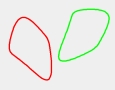
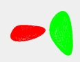
Figure 7: The "shape" of an HLJL particle, as scanned by second,
parallel HLJL body. An ellipse with the same axes is drawn in green.
|
The above expression for $r_{c}$ of HGO particles is a special case
of the "S function expansion" of pair properties for
nonspherical objects (Stone, Zewdie). In the most general case the
S-functions are combinations of three Wigner functions, but
symmetry often reduces this complexity (as here.)
|
|
| IV |
-
OUTLOOK (Pipedreams, rather)
-
The time evolution of orientations $\Omega_{1,2}$ is known even
for asymmetric tops (van Zon, Schofield)
-
The dependence of $r_{c}$ on $\Omega_{1,2}$ is known (see above)
so that $r_{c}$ may be reproduced quickly at simulation time
-
Thus $\tilde{d}(t)$ is known and may be used to
diagnose or predict events
-
Maybe one could approximate the non-algebraic function
$\tilde{d}(t)$ by a polynomial, Taylor or other? Then the root-finding
should be easier.
Here is a preliminary attempt at a Taylor expansion:
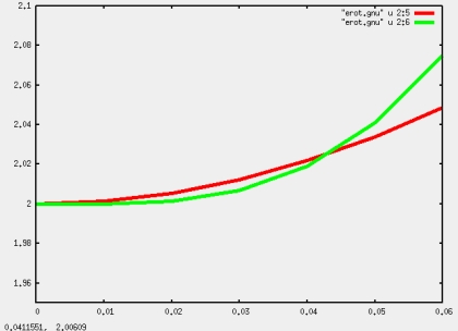
|
|
Figure 8: Taylor expansion of $\tilde{d}(t)$ for two
rotating ellipses
|
-
$r_{c}$ recovered from series expansions is of limited
accuracy. If that is not sufficient, the proposed method may
at least be used for container dynamics.
-
Containers may also be tailored to closely fit
complicated particles, sharing the inertial tensor of their content.
... and if all else fails:

|
|
vesely apr-2007
|
|