In many applications we encounter widely varying time scales. In such
cases the ``fast''_ degrees of freedom dominate the choice of
the time step, although they may be of lesser interest.
Example: A few slow-moving heavy ions in a bath of many light water
molecules.
Strategy: Mimick the effect of the secondary particles by suitably
sampled stochastic forces .
LANGEVIN'S equation of motion for a single ion in a viscous solvent:
(10.1)
where the statistical properties of the stochastic
acceleration
are
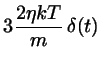
(10.2)
(10.3)
Explanation:
is not correlated to previous values of the ion velocity
Stochastic and frictional forces are mutually related
(both are caused by collisions of the ion with
solvent molecules)
Since equation 10.3 gives us only the a.c.f. of
,
we have yet to specify its statistical distribution; the usual choice
is a Gauss distribution for the components of
and similar for (t).
Subtracting
from
etc.,
we have
(10.4)
(10.5)
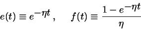
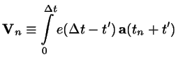
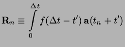
Defining
(10.6)
and
(10.7)
(10.8)
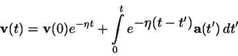
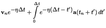
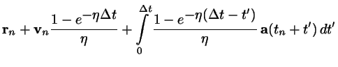
we may write the stepwise solution
(10.9)
(10.10)
The components of the stochastic vectors
are time integrals of the function
whose statistical properties
are given.
are themselves
random variates with known statistics:
,
, and
(10.11)
(10.12)
(10.13)
In the chapter about stochastics we described a method to produce
pairs of correlated Gaussian variates. We may apply this here to
generate and insert these in 10.9-10.10.
Generalization:
The stochastic force need not be -correlated.
If the solvent particles have a mass that is comparable with that of the
solute, they will also move with similar speeds. In such cases
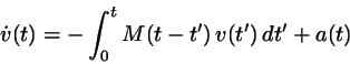
the generalized Langevin equation applies:
(10.14)
where
(10.15)
(10.16)
This is a stochastic integrodifferential equation involving
the ``history'' of the solute particle's motion in the form
of the memory function (see [MORI 65]).
Still, we may assume that decays fast.
Two approaches:
Approximate the memory function by a suitable class of functions:
assuming that the Laplace transform
may be represented
by a truncated chain fraction in the variable ,
the integrodifferential equation may be replaced by a set of coupled
differential equations. Written in matrix notation these equations have
the same form as 10.1 and may be treated accordingly.[VESELY 84]
Assume that may be neglected after
time steps.
Using a tabulated autocorrelation function one may generate an
autoregressive process by the method described in the chapter
on stochastics. By replacing the integral in 10.14 by a sum over
the most recent time steps, one arrives at a stepwise procedure
to produce
and
; see [SMITH 90], and also
[NILSSON 90]).
![$\displaystyle \frac{kT}{m}\left[ 1-e^{2}(\Delta t)\right]$](img683.png)
![$\displaystyle \frac{kT}{m \eta^{2}}
\left[ 2 \eta \Delta t - 3 + 4e(\Delta t) - e^{2}(\Delta t)\right]$](img685.png)
 may be represented
by a truncated chain fraction in the variable
may be represented
by a truncated chain fraction in the variable