8.1 Results of Linear Response Theory

We wish to develop relations between macroscopic transport coefficients and microscopic averages - which hopefully may be evaluated in simulation experiments.

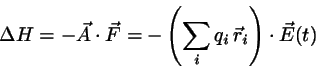
Let $H_{0}$ be the Hamiltonian of the given system when it is isolated. If we apply a weak disturbing field $F(t)$ that couples to some property $A(\Gamma)$ (with $<A>=0$) the Hamiltonian of the perturbed system is given by

$$H=H_{0}-A \cdot F(t)$$ (8.1)

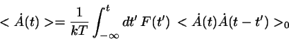
Linear response theory then leads to the following first order expression for the mean temporal change of $A$:

$$<\dot{A}(t)> = \frac{1}{kT} \int_{-\infty}^{t} dt' F(t') <\dot{A}(t)\dot{A}(t-t')>_{0}$$ (8.2)

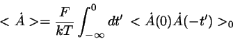
where the average $<>_{0}$ is to be taken over the unperturbed system. Assuming a constant field $F(t)=F$ switched on in the distant past we may write this as

$$<\dot{A}> = \frac{F}{kT} \int_{-\infty}^{0} dt' <\dot{A}(0)\dot{A}(-t')>_{0}$$ (8.3)

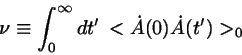
Independently, the fundamental Green-Kubo relations tell us that for any conserved quantity $A$ the appropriate transport coefficient is given by the equilibrium average

$$\nu \equiv \int_{0}^{\infty}dt' <\dot{A}(0)\dot{A}(t')>_{0}$$ (8.4)

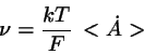
Combining this with the above equation we find that $<\dot{A}> = \frac{F}{kT} \nu$, or

$$\nu = \frac{kT}{F} <\dot{A}>$$ (8.5)

Thus we may determine the transport coefficient $\nu$ either from an equilibrium simulation using equ. 8.4, or from a non-equilibrium simulation with applied field using equ. 8.5 Generally the second method yields better statistics but is more prone to nonlinearity problems (large fields); also, systems responding to an external field must be thermostated.

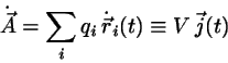
Example: Consider a fluid sample of ions in an electric field $\vec{F}(t)\equiv \vec{E}(t)$. The charge distribution is described by the quantity $\vec{A}(t) \equiv \sum_{i}q_{i} \vec{r}_{i}(t)$ which couples to the field according to

$$\Delta H = - \vec{A} \cdot \vec{F} = -\left( \sum_{i}q_{i} \vec{r}_{i}\right) \cdot \vec{E}(t)$$ (8.6)

The electrical current density $\vec{j}$ is defined by

$$\dot{\vec{A}} = \sum_{i}q_{i} \dot{\vec{r}}_{i}(t) \equiv V \vec{j}(t)$$ (8.7)

($V$ ... volume).

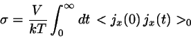
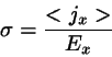
Now consider the conductivity $\sigma$. It may be determined in two ways:

• In an equilibrium simulation, using the Green-Kubo relation
  

  $$\sigma = \frac{V}{kT} \int_{0}^{\infty} dt <j_{x}(0) j_{x}(t)>_{0}$$ (8.8)

  
  

• In a non-equilibrium simulation, using the measured response to an applied field $\vec{E}=\{E_{x},0,0\}$:
  

  $$\sigma = \frac{<j_{x}>}{E_{x}}$$ (8.9)

  
  

Note: In the derivation of equ. 8.5 it is sufficient but not necessary that the external perturbation may be formulated as an additional term in the Hamiltonian. It is only necessary that the equations of motion contain perturbative terms which have to fulfill certain requirements. Specifically, the set

$$\dot{\vec{q}}_{i} = \vec{p}_{i} + A_{p} F(t)$$ (8.10)

$$\dot{\vec{p}}_{i} = \vec{K}_{i} + A_{q} F(t)$$ (8.11)

will be consistent with equ. 8.5 if only

$$\left( \vec{\nabla}_{q} \cdot A_{p}- \vec{\nabla}_{p} \cdot A_{q}\right) \cdot F(t)=0$$ (8.12)

(Note that we have switched to the Hamiltonian $q,p$ formalism.)

Example: In the Hamiltonian case $\Delta H = -A \cdot F$ the equations of motion are

$$\dot{\vec{q}} = \vec{\nabla}_{p} H = \vec{p}+\left( \vec{\nabla}_{p} A \right) \cdot F(t)$$ (8.13)

$$\dot{\vec{p}} = -\vec{\nabla}_{q} H = \vec{K} - \left( \vec{\nabla}_{q} A \right) \cdot F(t)$$ (8.14)

Therefore we have $A_{p}=\vec{\nabla}_{p}A$ and $A_{q}=\vec{\nabla}_{q}A$, and the requirement 8.12 is trivially fulfilled.