2.3 Starting configuration

On an Ising lattice, draw $N$ spin values with equal probabilities for $+ 1$ and $-1$.

Molecules in disordered media: Overlaps must be avoided. $\Longrightarrow$ Place the molecules on a lattice, then ``melt''this crystal before the actual simulation run: Thermalization.

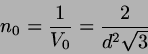
Population number in a cubic cell with face-centered cubic arrangement: $4m^{3}$, with $m=1,2,\dots$. Therefore typical particle numbers in simulations are $N= 32, 108, 256, 500$ etc.

What about 2-dimensional systems?

When simulating two-dimensional systems, the setting up of periodic base cells and of initial configurations is an issue that takes some considering. Since 2D systems are important both in the teaching and in the application of simulation, some suggestions are compiled here.

A dense packing of discs is hexagonal. The most convenient periodic cell in two dimensions would be quadratic. Unfortunately, these are contradictory requirements.

There are two possible periodic cells compatible with a hexagonal structure: (a) rectangular; (b) rhombic.

• Rectangular unit cell:

  Figure 2.2: 2D periodic cell: rectangle

  
  The unit cell then has $l_{y}=\sqrt{3} l_{x}$ and contains $N_{0}=2$ discs.
  
  Periodic boundary conditions are handled as usually, but with different base cell lengths along the axes: $L_{x}=m_{x} l_{x}$, $L_{y}=m_{y} l_{y}$ ($m_{x}$ may or may not be equal to $m_{y}$.)
  
  Nearest image convention: as usual, but again with different thresholds along the axes: $\pm L_{x}/2$ and $\pm L_{y}/2$, respectively.
  
  
• Rhombic unit cell:

  Figure 2.3: 2D periodic cell: rhombic

  
  The crystallographic unit is now a rhombus with $\alpha=60^{0}$ and $l_{y}=l_{x} \sqrt{3}/2$; it contains $N_{0}=1$ particle.
  
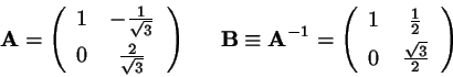
  Periodic boundary conditions are best handled in a non-orthogonal coordinate system. Let $\vec{r} \equiv \{x,y\}$ denote the cartesian coordinates, and $\vec{r}' \equiv \{x',y'\}$ the coordinates in the rhombic system. Then $\vec{r}' = \mbox{${\bf A}$} \cdot \vec{r}$ with
  

  $$\mbox{${\bf A}$} = \mbox{$\left( \begin{array}{cc}1&-\frac{1... ...2}\ \vspace{-9pt}\ 0&\frac{\sqrt{3}}{2}\end{array} \right)$}$$ (2.1)

  
  
  Specifically, when the new coordinates (after a time or MC step) are $x,y$, then
  • Compute
    

    $$x' = x-\frac{1}{\sqrt{3}} y$$ (2.2)

    $$y' = \frac{2}{\sqrt{3}} y$$ (2.3)

    
    

  • Apply PBC as always, but in rhombic coordinates:
    

    $$x' = (x'+2L_{x})\;{\rm mod} L_{x}$$ (2.4)

    $$y' = (y'+2L_{y})\;{\rm mod} L_{y}$$ (2.5)

    
    

  • Now transform back to Cartesius:
    

    $$x = x'+\frac{1}{2} y'$$ (2.6)

    $$y = \frac{\sqrt{3}}{2} y'$$ (2.7)

    
    

  Nearest image convention:
  Is applied in cartesian coordinates, possibly with a potential cutoff at $L_{y}/2$:
  

  $$\Delta x = \Delta x-L_{x} \;{\rm ANINT} (\Delta x/L_{x})$$ (2.8)

  $$\Delta y = \Delta y-L_{y} \;{\rm ANINT} (\Delta y/L_{y})$$ (2.9)

  
  

Reference Density in 2D: Let $d$ be a reference distance, which in the Lennard-Jones case is equal to $\left. \right.^{6}\!\!\sqrt{2} \sigma$, and for hard discs is identical to the disc diameter. The reference density is then

$$n_{0}=\frac{1}{V_{0}}=\frac{2}{d^{2}\sqrt{3}}$$ (2.10)

Let $n^{*}$ be a desired reduced density, $n^{*} \equiv n/n_{0} = V_{0}/V=d^{2}/l_{x}^{2}$. Thus, $l_{x}$ must be chosen as $l_{x}=d/\sqrt{n^{*}}$.



Adjusting density and temperature:
Given $N$, the density is adjusted to a desired value by shrinking or expanding the volume: scale all coordinates by a suitable factor.

The temperature is a constant parameter in an MC simulation. In molecular dynamics it must be adjusted in the following manner. Since

$$T=m \langle\vert\mbox{$\bf v$}\vert^{2} \rangle/3k$$

(with $k=1.3804 \cdot 10^{-23} J/deg$) or, in reduced units,

$$T^{*}=m^{*} \langle \vert\mbox{$\bf v$}^{*}\vert^{2} \rangle/3$$

we first take the average of $\vert\mbox{$\bf v$}^{*}\vert^{2}$ over a number of MD steps to determine the actual temperature of the simulated system. Then we scale each velocity component according to

$$v_{i,x} \leftrightarrow v_{i,x} \sqrt{T^{*}_{desired}/T^{*}_{actual}}$$

Since $T^{*}$ is a fluctuating quantity it can be adjusted only approximately.



EXERCISE: