


0.1 Definitions
Positions:  ,
,  with
with
 and
and
 ;
;
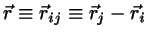
Interparticle unit vector:

Directions (unit vectors):  ,
, 
Width:
 (side-by-side),
Length:
(side-by-side),
Length:  (end-to-end).
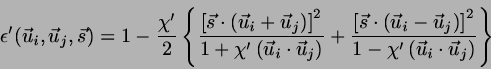
Then
![\begin{displaymath}
U\left(\vec{u}_{i},\vec{u}_{j},\vec{r}\right)
=4 \epsilon \l...
...i},\vec{u}_{j},\vec{s}\right)+\sigma_{0}}
\right]^{6}
\right\}
\end{displaymath}](img10.png) |
(1) |
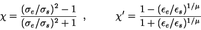
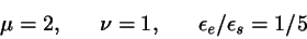
where the generalized diameter and well depth parameters are given by
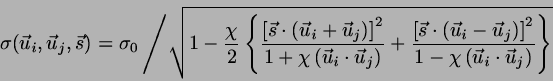 |
(2) |
and
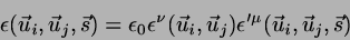 |
(3) |
with
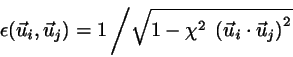 |
(4) |
 |
(5) |
and
 |
(6) |
A widely studied system is defined by the length-to-width ratio
 = 3. In this case the usual choice for the
parameters
= 3. In this case the usual choice for the
parameters  ,
,  and
and
 is
is
 |
(7) |
It should be noted that these parameters were identified by an optimal fit
to a site-site potential in which 4 LJ centers were placed along a line
at distances
 ; in other words, the distance between
the outer LJ centers was
; in other words, the distance between
the outer LJ centers was  .
.
For molecules of other l/w ratios other choices of the parameters would
be appropriate. However, model simulations are often done with the same
 , and even
.
, and even
.
For
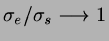 the model should become
identical to the simple LJ model; it does so only if the parameter
is also modified so as to approach
the model should become
identical to the simple LJ model; it does so only if the parameter
is also modified so as to approach  .
A simple linear interpolation formula would be
.
A simple linear interpolation formula would be
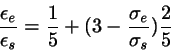 |
(8) |
The problem with this formula is that for lengths
 larger than
  it proceeds to unphysical
negative values of
. In fact, this ratio
should, for longer and longer molecules, asymptotically tend to zero, since
the negative side-by-side potential energy increases while the end-to-end
energy remains finite. An interpolation formula that accounts for this is
it proceeds to unphysical
negative values of
. In fact, this ratio
should, for longer and longer molecules, asymptotically tend to zero, since
the negative side-by-side potential energy increases while the end-to-end
energy remains finite. An interpolation formula that accounts for this is
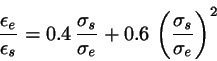 |
(9) |
F. J. Vesely / University of Vienna