| Franz J. Vesely > |
Weird bodies:
Franz J. Vesely franz.vesely@univie.ac.at Computational Physics Group, University of Vienna, Boltzmanngasse 5, A-1090 Vienna The task at hand is to characterize the shape of a body - for now, let it be a 2D contour. Of course, what we have in mind are hard body models of molecules, such as ellipses/oids, spherocylinders, spheroellipsoids. Molecular models are often rather symmetric and simple, but there is no harm in considering also more complex - weird - bodies, such as this one: 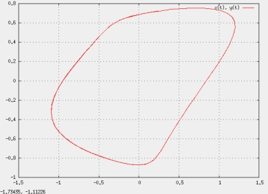
Figure 1: A weird 2D contour produced using three elliptic Fourier harmonics (see text.) An alternative that works even when the latter condition is not met, as with half-moon shaped bodies, is the elliptic Fourier analysis widely used in the biological sciences, morphology department. We will describe the elliptic Fourier method shortly, but first let us consider a possible application of any of these shape descriptors. Given two hard particles of given shape(s) and orientations it is possible to determine the contact distance as a function of both orientations. In 2D this may be written as $r_{c}(\theta_{1}, \theta_{2})$; in 3D it will be $r_{c}(\vec{\Omega}_{1},\vec{\Omega}_{2})$. The quantity $r_{c}$ may then be expanded in a double Fourier series (2D) or double spherical harmonics series (3D, linear particles). If $r_{c}$ is smooth, which it often is for convex molecular models, the series will converge fast, and thus the shape of the excluded volume between the two particles may be calculated quickly and handled efficiently. But the excluded volume is closely related to the hard body Mayer function, a key quantity in statistical mechanics. A particularly exciting prospect is the application of such descriptors in the currently re-emerging discipline of hard-body, or "event driven", molecular dynamics, EDMD. While in free flight, the particles simply fly straight and rotate, meaning that their orientations evolve linearly in time. The central task in EDMD, the detection of the very next collision, is then tantamount to finding the first zero line crossing of $r_{c}(t)-r(t)$, where $r(t)$ is the pair distance changing according to free flight motion. A quick calculation of $r_{c}(t)$ and, more importantly, its prognostication by a Taylor series in $t$ (if feasible) would be of great help. Now for the specific shape description used in biomorphology, the elliptic Fourier analysis (EFA). Recalling the parametric representation of an ellipse,
$
\begin{eqnarray}
x(t)&=&x_{0}+a_{11} \cos t + a_{12} \sin t
\;\;\;\;\;\; {\rm (1a)}
\\
y(t)&=&y_{0}+a_{21} \cos t + a_{22} \sin t
\;\;\;\;\;\; {\rm (1b)}
\end{eqnarray}
$
where $t \epsilon [0, 2 \pi ) $, we may generalize this to
$
\begin{eqnarray}
x(t)&=&x_{0}+ \sum \limits_{k=1}^{K} a_{1,2k-1} \cos k t + a_{1,2k} \sin kt
\;\;\;\;\;\; {\rm (2a)}
\\
y(t)&=&y_{0}+ \sum \limits_{k=1}^{K} a_{2,2k-1} \cos k t + a_{2,2k} \sin kt
\;\;\;\;\;\; {\rm (2b)}
\end{eqnarray}
$
More concisely, this is written as
$
r(t) - r_{0} = A \cdot w(t)
$
(3)
with $w(t)=[\cos t , \sin t, \cos 2t, \sin 2t, \dots ]$. In the simple ellipse case, $A$ may be inverted, and since the 2-vector $w$ is in this case of unit length (i.e. $w^{t} \cdot w = 1$) we find the alternative, non-parametric, representation of an ellipse,
$
\left( r - r_{0} \right)^{T} \cdot C \cdot \left( r - r_{0} \right)
=1
$
(4)
with $ C \equiv \left( A^{-1} \right)^{T} \cdot A^{-1} = \left( A^{-1} \right)^{2}$. However, in general the matrix $A$ is rectangular and therefore not invertible. Besides, the vector $w(t)$ is of length $K$. Let us return , then, to eq. (3). Taking the square of each side we find
$
\left| r(t) - r_{0} \right|^{2}
-
w^{T} \cdot A^{T} \cdot A \cdot w
=0
$
(5)
Now we interpret (5) as a constraint equation, $\sigma(r(t))=0$. Taking the gradient of $\sigma$ we have for the normal vector at the outline point $r(t)$ xxxxxxxxxxxxxxxxxx [... to be continued ...] |
franz vesely feb-07