3.3 Weighted density Approximations (WDA)

LDA and SGA must fail if the local density can achieve high values. For example, near a wall one may find density amplitudes in excess of homogeneous dense packing.

In such cases it is best to smear out the density over a small spatial region, using a suitable weighting function:

$${\rm\cal{F}}_{ex} [\rho ] = \int d\vec{r} \rho(\vec{r}) \Psi_{ex}(\bar{\rho}(\vec{r}))$$ (3.6)

where $\bar{\rho}(\vec{r})$ denotes the coarse-grained, or smoothed, or weighted density.

Various authors have contributed their specific recipes.

$\parbox{60pt}{ \includegraphics[width=54pt]{images/knot_1.ps} }$Nordholm and Tarazona I:

$${\rm\cal{F}}_{ex} [\rho ] = \int d\vec{r} \rho(\vec{r}) \Psi_{ex}(\bar{\rho}(\vec{r}))$$ (3.7)

$$\bar{\rho}(\vec{r}) = \int d \vec{r'} w_{0}(\vert\vec{r}-\vec{r'}\vert) \rho(\vec{r'})$$ (3.8)

$$w_{0} = \frac{3}{4 \pi \sigma^{3}} \Theta(\sigma-r)$$ (3.9)

For the excess free energy density NORDHOLM uses the excluded volume approximation

$$\beta \Psi_{ex}(\rho) = - \ln (1-\rho v_{0})$$ (3.10)

where $v_{0}=\sigma^{3}$ for hard spheres with diameter $\sigma$. An improvement introduced by TARAZONA is the use of the Carnahan-Starling approximation

$$\beta \Psi_{ex}(\rho) = \frac{\eta (4-3 \eta)}{(1-\eta)^{2}} \;\;\; {\rm with}\;\; \eta \equiv \frac{\pi \rho \sigma^{3}}{6}$$ (3.11)

$\parbox{60pt}{ \includegraphics[width=54pt]{images/knot_2.ps} }$Tarazona II:

$${\rm\cal{F}}_{ex} [\rho ] = \int d\vec{r} \rho(\vec{r}) \Psi_{ex}(\bar{\rho}(\vec{r}))$$ (3.12)

$$\bar{\rho}(\vec{r}) = \int d \vec{r'} w(\vert\vec{r}-\vec{r'}\vert;\bar{\rho}(\vec{r}))\rho(\vec{r'})$$ (3.13)

$$w(r;\rho) = w_{0}(r)+w_{1}(r) \rho + w_{2}(r) \rho^{2}$$ (3.14)

where $w_{0,1}$ is taken from a virial expansion of $c_{HS}^{(2)}(r;\rho)$, and $w_{2}$ from a fit to the PY solution.

$\parbox{60pt}{ \includegraphics[width=54pt]{images/knot_3.ps} }$Curtin-Ashcroft:

Similar to Tarazona II but with more effort regarding $w(r,\rho)$:

$${\rm\cal{F}}_{ex} [\rho ] = \int d\vec{r} \rho(\vec{r}) \Psi_{ex}(\bar{\rho}(\vec{r}))$$ (3.15)

$$\bar{\rho}(\vec{r}) = \int d \vec{r'} w(\vert\vec{r}-\vec{r'}\vert;\bar{\rho}(\vec{r}))\rho(\vec{r'})$$ (3.16)

and $w(r;\rho)$ such that with

$$c_{HS}^{(2)}(r;\rho) = -\beta \delta^{2}{\rm\cal F}_{ex} / \delta \rho(\vec{r}_{1}) \delta \rho(\vec{r}_{2})$$ (3.17)

it will produce the known pcf at all (homogeneous) densities.

Differenciating ${\rm\cal {F}}_{ex}[\rho ]$ twice by the argument $\rho$ one obtains

$$-\frac{1}{\beta} c^{(2)}(\rho;12) = 2 \Psi_{ex}'(\rho)w(12;\rho) +\rho \Psi_{ex}''(\rho) \int d\vec{3} w(13;\rho)w(32;\rho)$$

$$+ \rho \Psi_{ex}'(\rho) \int d\vec{3} \left[ w'(13;\rho)w(32;\rho)+w(13;\rho)w'(32;\rho) \right]$$ (3.18)

Various solution methods are possible. The standard procedure starts from a Fourier transform of this equation:

$$-\frac{1}{\beta} c_{k}^{(2)}(\rho)= 2 \Psi_{ex}'(\rho)w_{k}(\rho) \left[ \Psi'_{ex}(\rho) w_{k}^{2}(\rho) \right]$$ (3.19)

For given $c_{k}^{(2)}(\rho)$ (e. g. from Percus-Yevick) this equation may be solved numerically for $w(r;\rho)$.

DENTON and ASHCROFT generalized this procedure to mixtures.

$\parbox{60pt}{ \includegraphics[width=54pt]{images/knot_4.ps} }$Meister-Kroll; Groot-v.d. Eerden:
Let $\rho_{0}(\vec{r})$ be a ``coarse-grained'', slowly varying reference density. Expanding ${\rm\cal {F}}_{ex}[\rho ]$ around this reference density one finds

$${\rm\cal{F}}_{ex} [\rho ] = \int d\vec{r} \rho(\vec{r}) \Psi_{ex}(\rho_{0}(\vec{r}))$$ (3.20)

$$- \beta^{-1} \int d \vec{r} \int d \vec{r'} \rho(\vec{r}) L(\rho_{0}(\vec{r}); \vert\vec{r}-\vec{r'}\vert) (\rho(\vec{r'})-\rho_{0}(\vec{r}))$$ (3.21)

with

$$L(\rho_{0}(\vec{r}); \vert\vec{r}-\vec{r'}\vert) = \int_{0}^... ...c^{(2)} (\alpha \rho_{0}(\vec{r}); \vert\vec{r}-\vec{r'}\vert)$$ (3.22)

and

$$\rho_{0}(\vec{r}) = \int d \vec{r'} w(\vert\vec{r}-\vec{r'}\vert;\rho_{0}(\vec{r}))\rho(\vec{r'})$$ (3.23)

$$w(\vert\vec{r}-\vec{r'}\vert;\rho_{0}(\vec{r})) \equiv \frac... ...vec{r});\vert\vec{r}-\vec{r'}\vert)}{L_{0}(\rho_{0}(\vec{r}))}$$ (3.24)

$\parbox{60pt}{ \includegraphics[width=54pt]{images/knot_5.ps} }$Percus; Robledo-Varea:

Starting from equ. 2.15 we write

$${\rm\cal{F}}_{ex} [\rho ] = \int d\vec{r} \rho_{\sigma}(\vec{r}) \Psi_{ex}(\rho_{\tau}(\vec{r}))$$ (3.25)

where now $\rho_{\sigma}$ and $\rho_{\tau}$ are suitably averaged densities:

$$\rho_{\sigma}(\vec{r}) = \int d\vec{r}' \; \tilde{\sigma}(\vec{r}-\vec{r}')\; \rho(\vec{r}')$$ (3.26)

$$\rho_{\tau}(\vec{r}) = \int d\vec{r}' \; \tau(\vec{r}-\vec{r}')\; \rho(\vec{r}')$$ (3.27)

For the weighting functions $\tau$ und $\sigma$ Robledo and Varea suggest:

$$\tau(\vec{r}) = \frac{\Theta(\sigma/2-\vert\vec{r}\vert)}{\pi \sigma^{3}/6}$$ (3.28)

$$\tilde{\sigma}(\vec{r}) = \frac{\delta(\sigma/2-\vert\vec{r}\vert)}{\pi \sigma^{2}}$$ (3.29)

(Note that for the Tonks gas we have exactly $\tau(z)=\Theta(\sigma/2-\vert z\vert)/\sigma$ and $\tilde{\sigma}(z)=\delta(\sigma/2-\vert z\vert)/2$.)

$\parbox{60pt}{ \includegraphics[width=54pt]{images/knot_6.ps} }$Rosenfeld; Kierling-Rosinberg:

Rosenfeld studied mixtures of hard spheres with radii $R_{i}$. We restrict the discussion to one HS species, using the subsequently introduced formulation of Kierling und Rosinberg.

On the basis of geometric (overlap volume) consideration the following representation may be derived:

$$\beta {\rm\cal{F}}_{ex} [\{\rho(\vec{r})\} ]= \int d\vec{r}\; \Phi(\{n_{\alpha}(\vec{r})\})$$ (3.30)

where $n_{\alpha}$ are several averaged densities:

$$n_{\alpha}(\vec{r}) = \int d\vec{r}' \; \rho(\vec{r}') \omega^{(\alpha)}(\vec{r}-\vec{r}')$$ (3.31)

For the weighting functions $\omega^{(\alpha)}$, $\alpha=0,1,2,3$ Kierlik-Rosinberg find

$$\omega^{(3)}(r) = \Theta (R-r)$$ (3.32)

$$\omega^{(2)}(r) = \delta (R-r)$$ (3.33)

$$\omega^{(1)}(r) = \frac{1}{8\pi}\delta'(R-r)$$ (3.34)

$$\omega^{(0)}(r) = -\frac{1}{8\pi}\delta''(R-r) +\frac{1}{2\pi r}\delta'(R-r)$$ (3.35)

The choice of the quantities $\omega$ and the form of the function $\Phi$ follows from the requirement that in the homogeneous limit the PY equation is fulfilled:

$$\Phi(n_{0},n_{1},n_{2},n_{3}) = \Phi_{PY}= -n_{0} \ln (1-n_{... ...c{n_{1}n_{2}}{1-n_{3}} +\frac{n_{2}^{2}}{24 \pi (1-n_{3})^{2}}$$ (3.36)

$\parbox{60pt}{ \includegraphics[width=54pt]{images/knots_jf.ps} }$WDA in Perspective:

The WDAs given above are mostly based on heuristic arguments. For the ansatz of Meister-Kroll and Groot-v.d. Eerden it was shown by Fischer et al. that it is equivalent to the systematically derived Yvon-Born-Green approximation.

$\parbox{210pt}{ \includegraphics[width=180pt]{images/fischer_sok.ps} }$



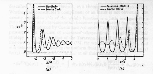
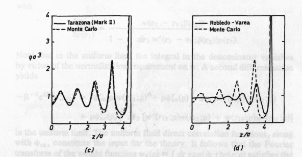
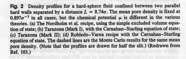
The application of various WDAs to the sample problem of hard spheres between two walls the following picrure emerges (from Evans 92):

$\parbox{60pt}{ \includegraphics[width=54pt]{images/knot_7.ps} }$Modified WDA:

Denton and Ashcroft suggested to apply a second averaging process to the ``weighted density'' $\bar{\rho}(\vec{r})$, this time averaging over the entire system. The resulting density $\hat{\rho}$ is then inserted in an expression for ${\rm\cal {F}}_{ex}[\rho ]$:

$$\frac{{\rm\cal{F}}_{ex} [\rho ]}{N} = \Psi_{ex}(\hat{\rho})$$ (3.37)

with

$$\hat{\rho} = \frac{1}{N} \int d\vec{r}\; \rho(\vec{r}) \; \i... ... \rho(\vec{r}') \hat{w}(\vert\vec{r}-\vec{r}'\vert;\hat{\rho})$$ (3.38)

The function $\hat{w}$ is chosen such that the above equations reproduce the correct direct pcf $c^{(2)}(\rho;r)$:

$$\hat{w}(r;\rho)=-\frac{1}{2\Psi_{ex}'(\rho)} \left[ kT \;c^{(2)}(\rho;r)+\frac{1}{V}\rho \Psi_{ex}''(\rho)\right]$$ (3.39)

If one uses the direct pcf and the free energy density $\Psi_{ex}$ according to Percus-Yevick the fluid-solid phase transition of hard spheres is well reproduced. Also, the enhomogeneous fluid density near a wall is well represented.

A similar ansatz is due to Lutsko and Baus. Their ``Generalized Effective Liquid Approximation'' (GELA) produces useful results at the freezing transition.