$ \vert p(y) dy \vert = \vert p(x)dx \vert $

$ p(y) = p(x) {\textstyle |} \frac{\textstyle dx}{\textstyle dy} | = p[f^{-1}(y)] \; | \frac{\textstyle df^{-1}(y)}{\textstyle dy} | $

$ I(\omega) = \frac{\textstyle \hbar \omega^{3}}{\textstyle \pi c^{3}} \frac{\textstyle 1}{\textstyle e^{\textstyle \hbar \omega/kT}-1} $

$ I(\lambda) = I[\omega(\lambda)] \; | \frac{\textstyle d \omega}{\textstyle d \lambda} | = \frac{\textstyle \hbar}{\textstyle \pi c^{3}} \left( \frac{\textstyle 2\pi c}{\textstyle \lambda} \right)^{3} \frac{\textstyle 1}{\textstyle e^{(hc/\lambda)/kT}-1} \left( \frac{\textstyle 2 \pi c}{\textstyle \lambda^{2}}\right) $

$ p(x) = c | \frac{\textstyle dy}{\textstyle dx} | = c | \frac{\textstyle df(x)}{\textstyle dx} | \;\;\;{\rm or} \;\;\; | \frac{\textstyle df(x)}{\textstyle dx} | = \frac{\textstyle 1}{\textstyle c} p(x) $

$ \begin{eqnarray} f(x) &=& P(x) \equiv \int \limits_{\textstyle a}^{\textstyle x} p(x') dx' \end{eqnarray} $

Transformation method: Let $p(x)$ be a desired density, with $y=P(x)=\int p(x') dx'$. Assume that $P^{-1}(y)$ be known. Sample $y$ from an equidistribution in the interval $(0,1)$. Compute $x=P^{-1}(y)$. The variable $x$ then has the desired probability density $p(x)$.

EXAMPLE: Let

Then $y = P (x)=1/2+(1/\pi) \arctan x$, with the inverse $P^{-1} (y)=\tan[\pi(y-1/2)]$. Therefore:

• Sample $y$ equidistributed in $(0,1)$.
• Compute $x=\tan[\pi(y-\frac{1}{2})]$.

Geometrical interpretation:
$y$ is sampled from an equidistribution $\in (0,1)$ and $x=P^{-1}(y)$.
$\Longrightarrow$ The regions where $P(x)$ is steeper (i.e. $p(x)$ is large) are hit more frequently.


EXERCISE: (See also here)

(a) Warm-up (no coding): A powder of approximately spherical metallic grains is used for sintering. The diameters of the grains obey a normal distribution with $\langle d \rangle =2 \mu m$ and $\sigma=0.25 \mu m$. Calculate the distribution of the grain volumes.

(b) Lorentzian density: Write a codelet which produces random variates with probability density


using the transformation method. Plot a frequency histogram of the produced random numbers and compare it with the given $p(x)$. Also, plot the distribution function $P(x)$ pertaining to the given density.

---

3.2.3 Generalized Transformation Method:

Same as before, but with n-tuples of random variates:
Let $x=(x_{1}, \dots ,x_{n})$, $x \epsilon D_{x}$, and $y= f(x)$ with $ y \epsilon D_{y}$. Then

($|\partial x/ \partial y|$ ... Jacobi determinant of the transformation $x= f^{-1}(y)$.) The following procedure for the production of Gaussian random variates may be understood as an application of this. $\Longrightarrow$

Normal distribution: ^3.1

Box-Muller technique: Sample $(y_{1},y_{2}) \in (0,1)^{2}$ Construct $ \begin{eqnarray} x_{1} & = & \sqrt{-2 \ln y_{1}} \cos 2 \pi y_{2} \\ x_{2} & = & \sqrt{-2 \ln y_{1}} \sin 2 \pi y_{2} \end{eqnarray} $ $x_{1},x_{2}$ are then normal-distributed and statistically independent. Gaussian variates with given variances $\sigma_{1}^{2}$, $\sigma_{2}^{2}$ are obtained by multiplying $x_{1}$ and $x_{2}$ by their respective $\sigma_{i}$.

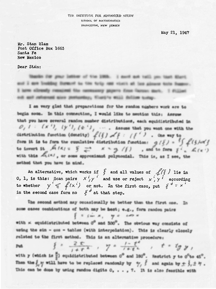
Footnote 3.1:

A "quick and dirty" method to produce almost normal variates goes as follows: if $y=x_{1}+\dots+x_{n}$ is the sum of $n=10 - 15$ equidistributed random numbers in $(-0.5,0.5)$, then the distribution of $z \equiv y\,\sqrt{12/n}$ is almost normal.

---

3.2.4 Rejection Method

A classic: created by John von Neumann, applicable to almost any $p(x)$.

Here is the original formulation:

     

And this is how we read it today:

Rejection method: Let $[a,b]$ be the allowed range of values of the variate $x$, and $p_{m}$ the maximum of the density $p(x)$. (1) Sample a pair of equidistributed random numbers, $x \in [a,b]$ and $y \in [0,p_{m}]$. (2) If $y \leq p(x)$, accept $x$ as the next random number, otherwise return to step 1.

The method is simple and fast, but it becomes inefficient whenever the area of the rectangle $[a,b] \otimes [0,p_{m}]$ is large compared to the area below the graph of $p(x)$ (which is, of course, equal to $1$.) In that case the "Improved Rejection Method" may be applicable: $\Longrightarrow$

Improved rejection method: Let $f(x)$ be a test function similar to $p(x)$, with $f(x) \geq p(x);\;\;\; x \in [a,b]$. $F(x) \equiv \int f(x)dx $ is assumed to be known and invertible (1) Pick a random number $x$ in $[a,b]$ from a distribution with density $ \bar{p}(x) = \frac{\textstyle f(x)}{\textstyle F(b)-F(a)} $ by using the transformation method. Pick an additional random number $y$ equidistributed in the interval $[0,f(x)]$. (2) If $y \leq p(x)$ accept $x$ as the next random number, else return to Step 1.

---

3.2.5 Multivariate Gaussian Distribution

$ p(x_{1}, \dots, x_{n}) = \frac{1}{\sqrt{\textstyle (2 \pi)^{n} S}} e^{\textstyle -\frac{1}{2} \sum \sum g_{ij} x_{i} x_{j}} $

or

$ \begin{eqnarray} p(x) & = & \frac{\textstyle1}{\textstyle\sqrt{(2 \pi)^{n} S}} e^{\textstyle -\frac{1}{2} x^{T} \cdot {G} \cdot x} \equiv \frac{1}{\sqrt{\textstyle (2 \pi)^{n}S}} e^{\textstyle -\frac{1}{2}Q} \end{eqnarray} $

with the covariance matrix of the $x_{i}$

$ \begin{eqnarray} S & \equiv & G^{-1} \equiv \left( \begin{array}{ccc} \langle x_{1}^{2} \rangle & \langle x_{1}x_{2} \rangle & \dots \\ \vdots & \langle x_{2}^{2} \rangle & \dots \\ & & \ddots \\ \end{array}\right) \end{eqnarray} $

$S \equiv | S|$ is the determinant of this matrix. $S$ and $G$ are symmetric, their eigenvalues are called $\sigma_{i}^{2}$ and $\gamma_{i}$ (sorry!).



EXAMPLE: Assume that two Gaussian variates have the variances $s_{11} \equiv \langle x_{1}^{2} \rangle =3$, $s_{22} \equiv \langle x_{2}^{2} \rangle =4$, and the covariance $s_{12} \equiv \langle x_{1}x_{2} \rangle =2$:

$ S = \left( \begin{array}{cc}3 & 2\\ \\2 & 4 \end{array} \right) ; \; \; G \equiv S^{-1} = \left( \begin{array}{cc} \frac{1}{2} & -\frac{1}{4} \\ \\ -\frac{1}{4} & \frac{3}{8}\end{array} \right) $

The quadratic form $Q$ in the exponent is then $Q=(1/2) x_{1}^{2} - (1/2)x_{1}x_{2} + (3/8)x_{2}^{2} $, and the lines of equal density (that is, of equal $Q$) are ellipses which are inclined with respect to the $x_{1,2}$ coordinate axes:
Rotate the axes of the ellipsoids $Q=const$ to coincide with the coordinate axes: $\Longrightarrow$ cross correlations vanish!

Principal axis transformation:

• Determine eigenvalues $\gamma_{j}$ and eigenvectors $g_{j}$ of $G$. (Use NAG-F02AMF, ESSL-SSYGV, or your own code.)
• Combine the n column vectors $g_{j}$ into a matrix $T$. This matrix diagonalizes $G$ (and consequently $Q$.)

Since $T$ is orthogonal ($T^{T}=T^{-1}$) it diagonalizes not only $G \equiv S^{-1}$ but also $S$ itself. $\Longrightarrow$ $S^{-1}$ need never be computed!

Having found $T$, we arrive at the following prescription for the production of correlated Gaussian variables: $\Longrightarrow$

Multivariate Gaussian distribution: Let the covariance matrix $S$ be given. Determine, by principal axis transformation, the diagonalization matrix $T$ for $S$ (This step is performed only once.) Generate $n$ mutually independent Gaussian random variates $y_{i}$ with the variances $\sigma_{i}^{2}$. Transform the vector $y \equiv (y_{1} \dots y_{n})^{T}$ according to $ \begin{eqnarray} x&=& T \cdot y \end{eqnarray} $ The $n$ elements of the vector $x$ are then random numbers obeying the desired distribution.

Let's try it out...


EXAMPLE: Once more, let

$ S=\left( \begin{array}{cc}3 & 2\\ \\2 & 4\end{array} \right) , \;\; {\rm with\; the\; inverse}\;\; G=\left( \begin{array}{cc}\frac{1}{2}& - \frac{1}{4}\\ \\-\frac{1}{4} & \frac{3}{8}\end{array} \right) $

Principal axis transformation: The eigenvalues of $S$ are $\sigma_{1,2}^{2}= (7\pm\sqrt{17})/2 = 5.562|1.438$, and the corresponding eigenvectors are

$ s_{1}=\left( \begin{array}{r} 0.615 \\ \\0.788 \end{array} \right) \;\;\;\;\; s_{2}=\left( \begin{array}{r} 0.788 \\ \\-0.615 \end{array} \right) \;\;\;\;\; {\rm Thus}\;\;\;\;\; T=\left( \begin{array}{cc}0.615 & 0.788\\ \\0.788 & -0.615\end{array} \right) $

Generator: To produce pairs $(x_{1},x_{2})$ of Gaussian random numbers with the given covariance matrix:

• Draw $y_{1}$ and $y_{2}$ Gaussian, uncorrelated, with variances $5.562$ and $1.438$.
  
• Compute $x_{1}$ and $x_{2}$ according to
  
  $ \left( \begin{array}{r} x_{1} \\ \\x_{2} \end{array} \right)= \left( \begin{array}{cc}0.615 & 0.788\\ \\0.788 & -0.615 \end{array} \right) \cdot \left( \begin{array}{r} y_{1} \\ \\y_{2} \end{array} \right) $
  
  

EXERCISE:
(See also here)
Write a program that generates a sequence of bivariate Gaussian random numbers with the statistical properties as assumed in the foregoing example. Determine $\langle x_{1}^{2}\rangle$, $\langle x_{2}^{2}\rangle$, and $\langle x_{1}x_{2}\rangle$ to see if they indeed approach the given values of $3$, $4$, and $2$.

---

3.2.6 Homogeneous distributions in Orientation Space

Equidistribution on the unit circle: Draw a pair of equidistributed random numbers $(y_{1},y_{2})$ $\in (-1,1)^{2}$; compute $r^{2} = y_{1}^{2}+y_{2}^{2}$; if necessary, repeat until $r^{2} \leq 1$. $x_{1} \equiv y_{1}/r$ and $x_{2} \equiv y_{2}/r$ are the cartesian coordinates of points that are homogeneously distributed on the circumference of the unit circle.

Fig. 3.7: Simple as can be...

Equidistribution on a spherical surface: Draw pairs of random numbers $(y_{1},y_{2})$ $\in (-1,1)^{2}$ until $r^{2} \equiv $ ${y_{1}^{2}+y_{2}^{2}} \leq 1$. The quantities $ \begin{eqnarray} x_{1} &= & 2y_{1} \sqrt{1-r^{2}} \\ x_{2} &= & 2y_{2} \sqrt{1-r^{2}} \\ x_{3} &= & 1-2r^{2} \end{eqnarray} $ are then the cartesian coordinates of points from a homogeneous distribution on the surface of the unit sphere.

Fig. 3.8: More refined: Marsaglia's recipe

(Generalization to hyperspherical surfaces: see Vesely, Comp. Phys..)

---

vesely 2005-10-10

<

>