4.1.3 Explicit Methods

- Euler-Cauchy (from DNGF; see above)

- Leapfrog algorithm (from DST):

$$\mbox{$\bf y$}_{n+1} = \mbox{$\bf y$}_{n-1}+\mbox{$\bf f$}_{n}\, 2\Delta t + O[(\Delta t)^{3}]$$

$$\mbox{$\bf y$}_{n+2} = \mbox{$\bf y$}_{n}+\mbox{$\bf f$}_{n+1}\, 2\Delta t + O[(\Delta t)^{3}]$$

This is an example of a multistep technique, as timesteps $t_{n}$ and $t_{n-1}$ contribute $y(t_{n+1})$. Stability analysis for such algorithms is as follows:

Let the explicit multistep scheme be written as

$$\mbox{$\bf y$}_{n+1}=\sum_{j=0}^{k} \left[ a_{j}\mbox{$\bf y$}_{n-j}+b_{j}\Delta t \,\mbox{$\bf f$}_{n-j} \right]$$

Inserting a slightly deviating solution $\mbox{$\bf y$}_{n-j}+\mbox{$\bf e$}_{n-j}$ and computing the difference, we have

$$\mbox{$\bf e$}_{n+1} \approx \sum_{j=0}^{k} \left[ a_{j} \mb... ...\sum_{j=0}^{k} \mbox{${\bf A}$}_{j} \cdot \mbox{$\bf e$}_{n-j}$$

We combine the errors at subsequent time steps to a vector

$$\mbox{$\bf\mbox{\boldmath$\eta$}$}_{n} \equiv \left( \begin... ...$}_{n-1} \\ \vdots \\ \mbox{$\bf e$}_{n-k} \end{array} \right)$$

and define the quadratic matrix

$$\mbox{${\bf G}$} \equiv \left( \begin{array}{cccc} \mbox{${... ...0 \\ 0 & \dots & \mbox{${\bf I}$}& 0 \\ \end{array}\right)$$

Then

$$\mbox{$\bf\mbox{\boldmath$\eta$}$}_{n+1}= \mbox{${\bf G}$} \cdot \mbox{$\bf\mbox{\boldmath$\eta$}$}_{n}$$

Stability is guaranteed if

$$\vert g_{i}\vert\leq 1 \,,\;\; {\rm for\; all \; \it i}$$

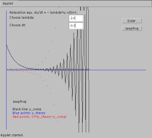
EXAMPLE 1: Leapfrog / Relaxation equation:

$$y_{n+1}=y_{n-1}-2\Delta t \lambda y_{n} +O[(\Delta t)^{3}]$$

Therefore

$$e_{n+1} \approx -2\Delta t \lambda e_{n} + e_{n-1}$$

which means that $A_{0}=-2\Delta t \lambda$, and $A_{1}=1$, and the matrix $\mbox{${\bf G}$}$ is

$$\mbox{${\bf G}$}=\mbox{$\left( \begin{array}{cc}-2\Delta t \lambda&1\\ \vspace{-9pt}\\ 1&0\end{array} \right)$}$$

with eigenvalues

$$g_{1,2}=-\lambda \Delta t \pm \sqrt{(\lambda \Delta t)^{2}+1}$$

For real $\lambda \Delta t$ we find that $\vert g_{2}\vert > 1$ always, meaning that the leapfrog scheme is unstable for the relaxation (or growth) equation.

Relaxation equation: Euler / Leapfrog:
Start Applet

EXAMPLE 2: Leapfrog / Harmonic oscillator:

$$\mbox{$\bf y$}_{n+1}=2\Delta t \, \mbox{${\bf L}$} \cdot \mbox{$\bf y$}_{n} + \mbox{$\bf y$}_{n-1}$$

and

$$\mbox{$\bf e$}_{n+1} \approx 2\Delta t \, \mbox{${\bf L}$} \cdot \mbox{$\bf e$}_{n} + \mbox{$\bf e$}_{n-1}$$

For the amplification matrix we find (with $\alpha \equiv 2 \Delta t$)

$$\mbox{${\bf G}$} = \mbox{$\left( \begin{array}{cc}\alpha \mb... ... & 1 \\ 1 & 0 & 0 & 0 \\ 0 & 1 & 0 & 0 \end{array}\right)$$

with eigenvalues

$$g= \pm \left[ (1-\frac{\alpha^{2} \omega_{0}^{2}}{2}) \pm i ... ...\sqrt{1-\frac{\alpha^{2} \omega_{0}^{2}}{4}} \; \right]^{1/2}$$

But the modulus of this is always $\vert g\vert=1$. $\Longrightarrow$The leapfrog algorithm is marginally stable for the harmonic oscillator.