2.3.2 Jacobi Relaxation

Divide the given matrix according to $\mbox{${\bf A}$}=\mbox{${\bf D}$}+\mbox{${\bf L}$}+\mbox{${\bf R}$}$ where $\mbox{${\bf D}$}$ contains only the diagonal elements of $\mbox{${\bf A}$}$, while $\mbox{${\bf L}$}$ and $\mbox{${\bf R}$}$ are the left and right parts of $\mbox{${\bf A}$}$, respectively.

Choose $\mbox{${\bf B}$}=\mbox{${\bf D}$}$ and write the iteration formula as

$$\fbox{ $ \mbox{${\bf D}$} \cdot \mbox{$\bf x$}_{k+1}=\mbox{$\bf b$}+\left[\mbox{${\bf D}$}-\mbox{${\bf A}$}\right] \cdot \mbox{$\bf x$}_{k} $ }$$

or

$$a_{ii} \, x_{i}^{(k+1)} = b_{i}-\sum_{j \neq i}a_{ij}\,x_{j}^{(k)}\, ; \;\;\; i=1,\dots,N$$

EXAMPLE: In $\mbox{${\bf A}$} \cdot \mbox{$\bf x$}=\mbox{$\bf b$}$ let

$$\mbox{${\bf A}$}=\mbox{$\left( \begin{array}{cc}3&1\\ \vspac... ...\begin{array}{r} 3 \\ \vspace{-9 pt}\\ 2 \end{array} \right)$}$$

Starting from the estimated solution

$$\mbox{$\bf x$}_{0}=\mbox{$\left( \begin{array}{r} 1.2 \\ \vspace{-9 pt}\\ 0.2 \end{array} \right)$}$$

and using the diagonal part of $\mbox{${\bf A}$}$,

$$\mbox{${\bf D}$}=\mbox{$\left( \begin{array}{cc}3&0\\ \vspace{-9pt}\\ 0&4\end{array} \right)$}$$

in the iteration we find the increasingly more accurate solutions

$$\mbox{$\bf x$}_{1}= \mbox{$\left( \begin{array}{r} 0.933 \\ ... ...\begin{array}{r} 1 \\ \vspace{-9 pt}\\ 0 \end{array} \right)$}$$

Convergence rate:

Writing the Jacobi scheme in the form

$$\mbox{$\bf x$}_{k+1} = \mbox{${\bf D}$}^{-1} \cdot \mbox{$\bf b$}+ \mbox{${\bf D}$}^{-1}... ...{${\bf D}$}^{-1} \cdot \mbox{$\bf b$}+\mbox{${\bf J}$} \cdot \mbox{$\bf x$}_{k}$$

with the Jacobi block matrix

$$\mbox{${\bf J}$} \equiv \mbox{${\bf D}$}^{-1} \cdot \left[ \mbox{${\bf D}$}-\mbox{${\bf A... ...] =-\mbox{${\bf D}$}^{-1} \cdot \left[ \mbox{${\bf L}$}+\mbox{${\bf R}$}\right]$$

convergence requires that all eigenvalues of $\mbox{${\bf J}$}$ be smaller than one (by absolute value). Denoting the largest eigenvalue (the spectral radius) of $\mbox{${\bf J}$}$ by $\lambda_{J}$, we have for the asymptotic rate of convergence

$$r_{J} \equiv \frac{\left\vert \mbox{$\bf x$}_{k+1}-\mbox{$\bf x$}_{k}\right\ve... ...x$}_{k}-\mbox{$\bf x$} \right\vert} \approx \left\vert \lambda_{J}-1\right\vert$$

In the above example $\lambda_{J}=0.408$ and $r \approx 0.59$.

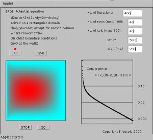
The electrostatic problem shown before was treated by Jacobi iteration:

Start Applet