


Next: 1.3.3 First derivatives in
Up: 1.3 Difference Quotients
Previous: 1.3.1 First Derivatives
The same procedure as before yields
DDNGF:
Example:
Let's try again....
DDNGB:
Example:
And the winner is...
DDST:
Example:
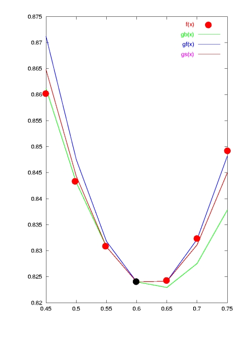
Figure: Interpolation, including first and second derivatives as
approximated by backward (blue), forward (green) and
Stirling (red) differencing. In the neighborhood of  (black dot) the tabulated function is best represented by Stirling.
The interpolation curves are actually parabolas, but as only their
values at
(black dot) the tabulated function is best represented by Stirling.
The interpolation curves are actually parabolas, but as only their
values at  are of interest they are drawn as broken
lines.
are of interest they are drawn as broken
lines.
Next: 1.3.3 First derivatives in
Up: 1.3 Difference Quotients
Previous: 1.3.1 First Derivatives
Franz J. Vesely Oct 2005
See also: "Computational Physics - An Introduction," Kluwer-Plenum 2001
![$\displaystyle \frac{1}{(\Delta x)^{2}} \left[ \Delta^{2} \mbox{$f_{k}$}
- \Delta^{3} \mbox{$f_{k}$}+ \frac{11}{12} \Delta^{4} \mbox{$f_{k}$}- \dots \right]$](img98.png)

![$\displaystyle \frac{1}{(\Delta x)^{2}} \left[ f_{k+2}-2f_{k+1}+f_{k}\right]
+ O(\Delta x)$](img100.png)
![$\displaystyle \frac{1}{(\Delta x)^{2}}
\left[ \nabla^{2} \mbox{$f_{k}$}
+ \nabla^{3} \mbox{$f_{k}$}+ \frac{11}{12} \nabla^{4} \mbox{$f_{k}$}+ \dots \right]$](img102.png)

![$\displaystyle \frac{1}{(\Delta x)^{2}} \left[ f_{k}-2f_{k-1}+f_{k-2}\right]
+ O(\Delta x)$](img104.png)
![$\displaystyle \frac{1}{(\Delta x)^{2}} \left[ \delta^{2} \mbox{$f_{k}$}- \frac{...
...elta^{4} \mbox{$f_{k}$}
+ \frac{1}{90} \delta^{6} \mbox{$f_{k}$}- \dots \right]$](img106.png)
![$\displaystyle \frac{1}{(\Delta x)^{2}} \delta^{2} \mbox{$f_{k}$}
+ O\left[(\Delta x)^{2}\right]$](img107.png)
![$\displaystyle \frac{1}{(\Delta x)^{2}} \left[ f_{k+1}-2f_{k}+f_{k-1}\right]
+ O\left[(\Delta x)^{2}\right]$](img108.png)