| Franz J. Vesely > MolSim Tutorial > NEMD I: Non-Hamiltonian Mthods |
5 Molecular Dynamics far from EquilibriumThere are at least two good reasons to study non-equilibrium systems:
Subsections
We wish to develop relations between macroscopic transport coefficients
and microscopic averages - which hopefully may be evaluated in
simulation experiments.
|
| $ \nu \equiv \int_{0}^{\infty}dt' <\dot{A}(0)\dot{A}(t')>_{0} $ | (2) |
$
\nu = \frac{\textstyle kT}{\textstyle F} <\dot{A}>
$
Thus we may determine the transport coefficient $\nu$
either from an equilibrium simulation using equ.
2, or from a non-equilibrium
simulation with applied field using equ.
1
Generally the second method yields better statistics but is more prone
to nonlinearity problems (large fields); also, systems responding to an
external field must be thermostated.
Example: Consider a fluid sample of ions in an electric field $\vec{F}(t)\equiv \vec{E}(t)$. The charge distribution is described by the quantity $\vec{A}(t) \equiv \sum_{i}q_{i}\vec{r}_{i}(t)$ which couples to the field according to
$
\Delta H = - \vec{A} \cdot \vec{F}
= -\left( \sum_{i}q_{i} \vec{r}_{i}\right) \cdot \vec{E}(t)
$
The electrical current density $\vec{j}$ is defined by
$
\dot{\vec{A}} = \sum_{i}q_{i} \dot{\vec{r}}_{i}(t)
\equiv V \vec{j}(t)
$
($V$... volume).
Now consider the conductivity $\sigma$. It may be determined in two ways:
- In an equilibrium simulation, using the Green-Kubo relation
$ \sigma = \frac{\textstyle 1}{\textstyle kT} \int_{0}^{\infty} dt < j_{x}(0) j_{x}(t) >_{0} $
- In a non-equilibrium simulation, using the measured response to an applied
field $\vec{E}=\{E_{x},0,0\}$:
$ \sigma = \frac{\textstyle < j_{x} > }{\textstyle E_{x}} $
$
\begin{eqnarray}
\dot{\vec{q}}_{i} &=& \vec{p}_{i} + A_{p} F(t)
\\
\dot{\vec{p}}_{i} &=& \vec{K}_{i} + A_{q} F(t)
\end{eqnarray}
$
will be consistent with equ. 1 if only
$
\left( \vec{\nabla}_{q} \cdot A_{p}-
\vec{\nabla}_{p} \cdot A_{q}\right) \cdot F(t)=0
$
(Note that we have switched to the Hamiltonian $q,p$ formalism.)
Example: In the Hamiltonian case $\Delta H = -A \cdot F$ the equations of motion are
$ \begin{eqnarray}
\dot{\vec{q}} &=& \vec{\nabla}_{p} H =
\vec{p}+\left( \vec{\nabla}_{p} A \right) \cdot F(t)
\\
\dot{\vec{p}} &=& -\vec{\nabla}_{q} H =
\vec{K} + \left( \vec{\nabla}_{q} A \right) \cdot F(t)
\end{eqnarray} $
Therefore we have $A_{p}=\vec{\nabla}_{p}A$ and $A_{q}=\vec{\nabla}_{q}A$, and the requirement 3 is trivially fulfilled.
Viscosity: Non-Hamiltonian methods
Subsections
Gosling and Singer
[Mol.Phys.26(1973)1475]An external force $\vec{F}=\{F_{x},0,0\}$ is introduced in the equations of motion according to
$
F_{i,x}=F_{0}\sin k z_{i} \;\;\;\;{\rm with}\;\;\;\;
k\equiv 2 \pi \frac{\textstyle m}{\textstyle L}; \;\; m=1,2,\dots
$
(Note: $\vec{A}_{q}=\{\sin kz, 0, 0 \}$ and $\vec{A}_{p}=0$ which fulfills
3.)
This will eventually lead to an average velocity profile which theoretically should look like
$
< v_{i,x} > =\frac{\textstyle n}{\textstyle k^{2}\eta} F_{0} \sin kz_{i}=v_{0} \sin kz_{i}
$
where $n \equiv N/V$.
Fitting the actual velocity profile to this expression we find $v_{0}$
and from that the $k$-dependent viscosity:
$
\eta(k)=\frac{\textstyle nF_{0}}{\textstyle v_{0}k^{2}}
$
Repeating the calculation for several values of $k$
and extrapolating to $k \rightarrow 0$
we find an estimate for $\eta \equiv \eta(k=0)$
Note: The applied force does work against the viscous forces, thus inducing an undesirable temperature rise.
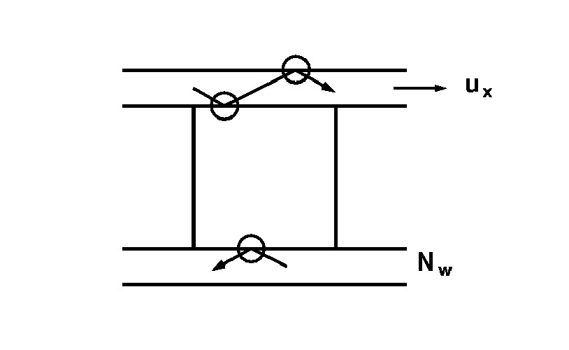
Ashurst and Hoover
[Phys.Rev.Lett 31(1973)206]These authors use periodic boundary conditions in the $x,y$ directions; the upper and lower boundaries are replaced by layers containing trapped particles. The upper layer has a mean velocity $u_{x}$ while the bottom layer is at rest.
|
The desired shear rate is $\gamma = u_{x}/L$. We need an external force
$
\vec{F}(t)=-\sum_{i}^{N_{w}}\sum_{j}^{N} \vec{K}_{ij}(t)/N_{w}
$
to achieve this. This force is proportional to the viscosity.
Again, the temperature will slowly increase due to the work done by the external force.
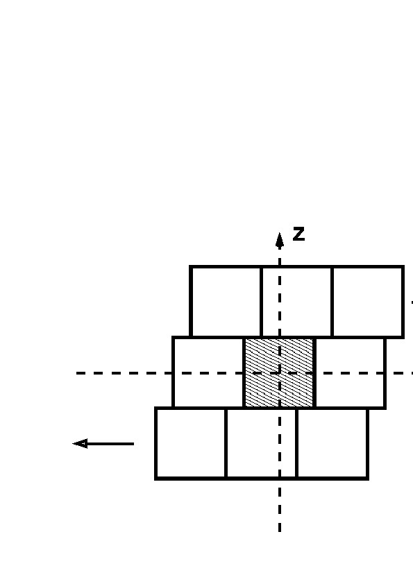
Lees and Edwards
[Lees+Edwards, J.Phys.C 5(1972)1921; Evans-Morriss Mol.Phys. 37(1979)1745; Comp.Phys.Rep. 1(1984)297]Lees and Edwards suggested a method to combine laminary flow with periodic boundaries in the $z$ direction:
|
Here are in language-independent form, the appropriate code parts for PBC and NIC:
// Periodic boundary conditions:
// round(float) is the integer next to float
// L is the cell side length; note that x,y,z vary between -L/2 and L/2
// t is the elapsed time
// gamma is the shear rate
       cz=round(z/L)
       cx=x-cz*gamma*L*t
       x=cx-round(x/L)*L
       y=y-round(y/L)*L
       z=z-cz*L
       .....
// Nearest image convention:
       delx=x(j)-x(i)
       ...
       cz=round(dz/L)
       cdelx=delx-cz*gamma*L*t
       delx=cdelx-round(cdelx/L)*L
       dely=dely-round(dely/L)*L
       delz=delz-cz*L
       ...
This is the procedure for a single time step:
- Compute all forces, applying the nearest image convention
- Integrate the equs. of motion for $t_{n} \rightarrow t_{n+1}$
- Perform a least squares fit to a linear velocity profile,
determining $u_{0}$ and $\gamma'$ such that
$ v_{i,x}=u_{0}+\gamma' \left( z_{i}\right) + c_{i,x} $where $c_{i,x}$ is the thermal velocity of the particle.
- Apply a simple thermostat by adjusting all $v_{i,x},v_{i,y}$
such that
$ \sum_{i} \frac{\textstyle m}{\textstyle 2}\left( v_{i,x}^{2}+v_{i,y}^{2}\right)=NkT $
- Compute the stress tensor element
$ \sigma_{xz} \equiv \sum_{i} \left[ m v_{i,x} v_{i,z}+K_{i,x} z_{i} \right] $
$
<\sigma_{xz}>=-\eta \gamma
$
vesely may-06
| < | > |