To avoid the handling of small numbers, choose units appropriate to
the model.
Lennard-Jones:
Energy unit $E_{0}=\epsilon$; length $l_{0}=\sigma$.
The pair energy is then
$
u_{LJ}^{*}=4\left[ r^{*-12}-r^{*-6}\right]
$
where $u^{*} \equiv u/\epsilon$ and $r^{*} \equiv r/\sigma$.
As the third mechanical unit, choose the atomic mass
$m_{0}=1 AMU= 1.6606 \cdot 10^{-27}kg$.
The time unit is now the combination $t_{0}=\sqrt{m_{0} \sigma^{2}/\epsilon}$.
Electrical charge: best measured in multiples of the
electron charge, $q_{0}=1.602 \cdot 10^{-19} As$.
Number density:
$\rho=N/V$ is a large number; therefore we
reduce it by a suitable standard density, $\rho_{0}=1/\sigma^{3}$:
$\rho^{*} \equiv N \sigma^{3}/V$.
Temperature: $T_{0}=\epsilon/k$
Hard spheres:
no "natural" unit of energy; therefore choose
self-consistent time unit $t_{0}=\sqrt{m_{0}d^{2}/kT}$.
For hard spheres of diameter $d_{0}=2 r_{0}$ the customary
standard density is $\rho_{0}=\sqrt{2}/d_{0}^{3}$; thus:
$\rho^{*}=N d_{0}^{3}/V\sqrt{2}$.
Approximately 95 pc. of the computing time in a simulation is expended for
the calculation of the pair forces, torques, energies etc. For systems
of more than $N=500$ particles the interaction is usually cut off at some
pair distance smaller than half the box side length: $r_{co}<L/2$.
Even the scanning of all particle pairs for the condition
$r_{ij}^{2} < r_{co}^{2}$ may become costly for large systems.
Verlet suggested that in such cases the possible interaction partners
of each particle $i$ are listed in an array, and only the particles in
that list are considered. As the molecules diffuse around, the lists
must be updated regularly by an occasional $N(N-1)/2$ scan. Here is the
detailed procedure:
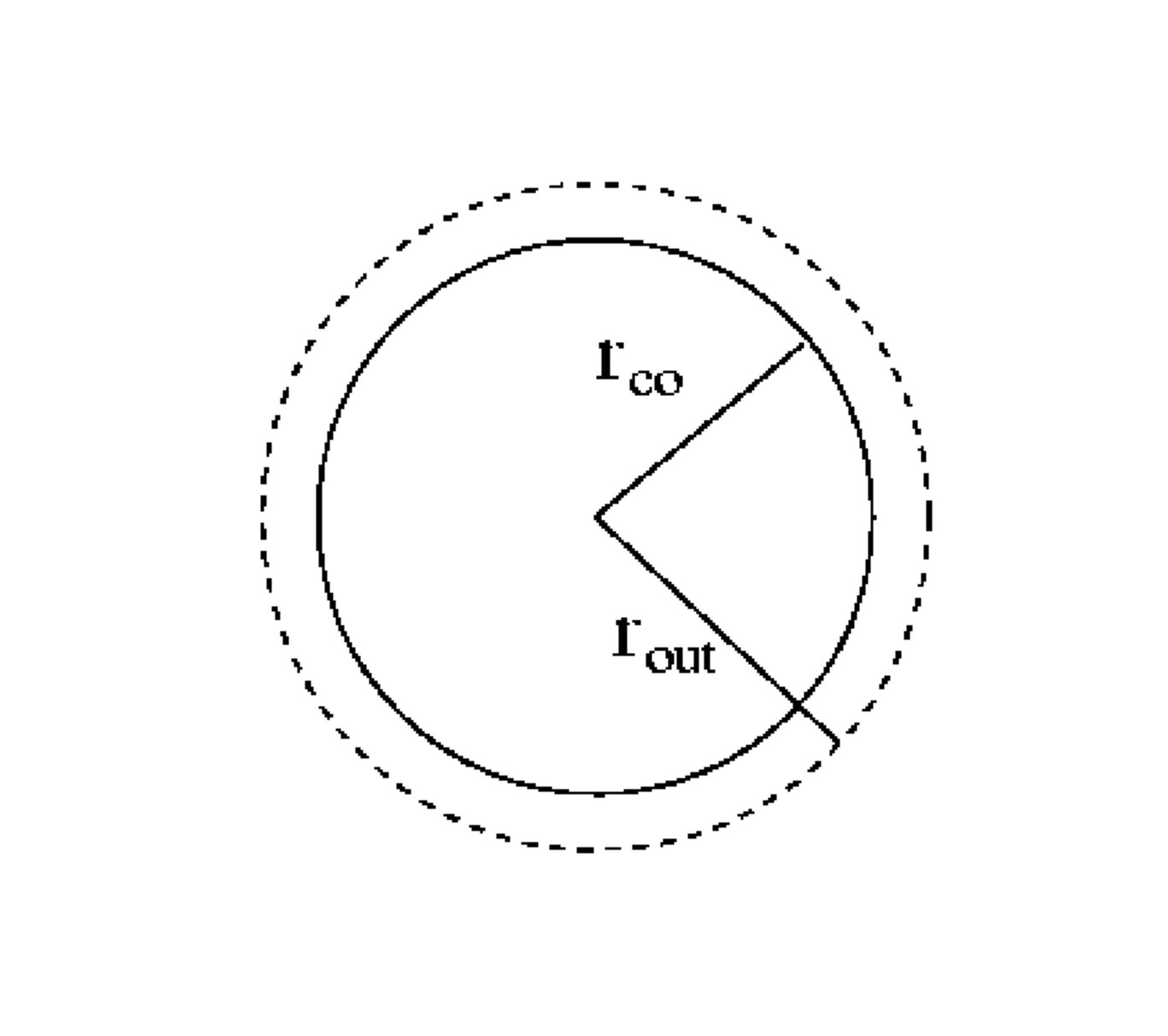
Figure 1.4:
Verlet neighbour lists: $r_{out} \approx 1.1-1.2 r_{co}$.
All particles $j$ within a distance $r_{out}$ of particle $i$
are entered in a list.
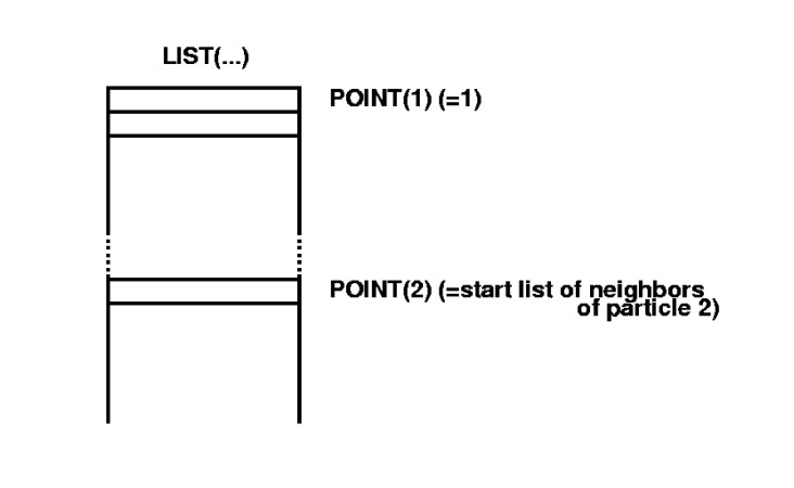
These lists of neighbours, $LIST(i)$, are stored in sequence, in one long
array. For each $i$ a pointer $POINT(i)$ points to the start of
the list of its neighbours:
Figure 1.5:
Storage of Verlet lists
The first setup of the lists requires $N(N-1)$ operations; every
10-20 steps the lists must be updated, again at the same cost.
However, in the time of diffusion between $r_{co}$ and $r_{out}$,
for each particle $i$ only the possible partners with indices
$j=LIST(POINT(i))$ to $j=LIST(POINT(i+1)-1)$ need be considered.
1.2.5 Linked lists
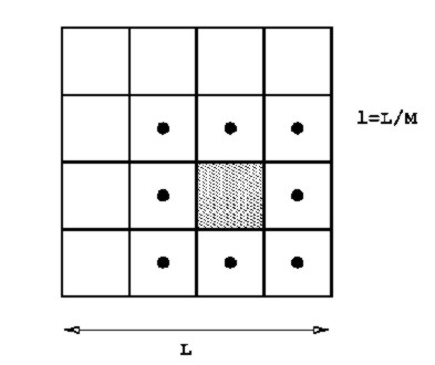
For even larger particle numbers the cell volume $L^{3}$
is divided into $M^{3}$ subcells with side lengths $l \equiv L/M \leq r_{co}$.
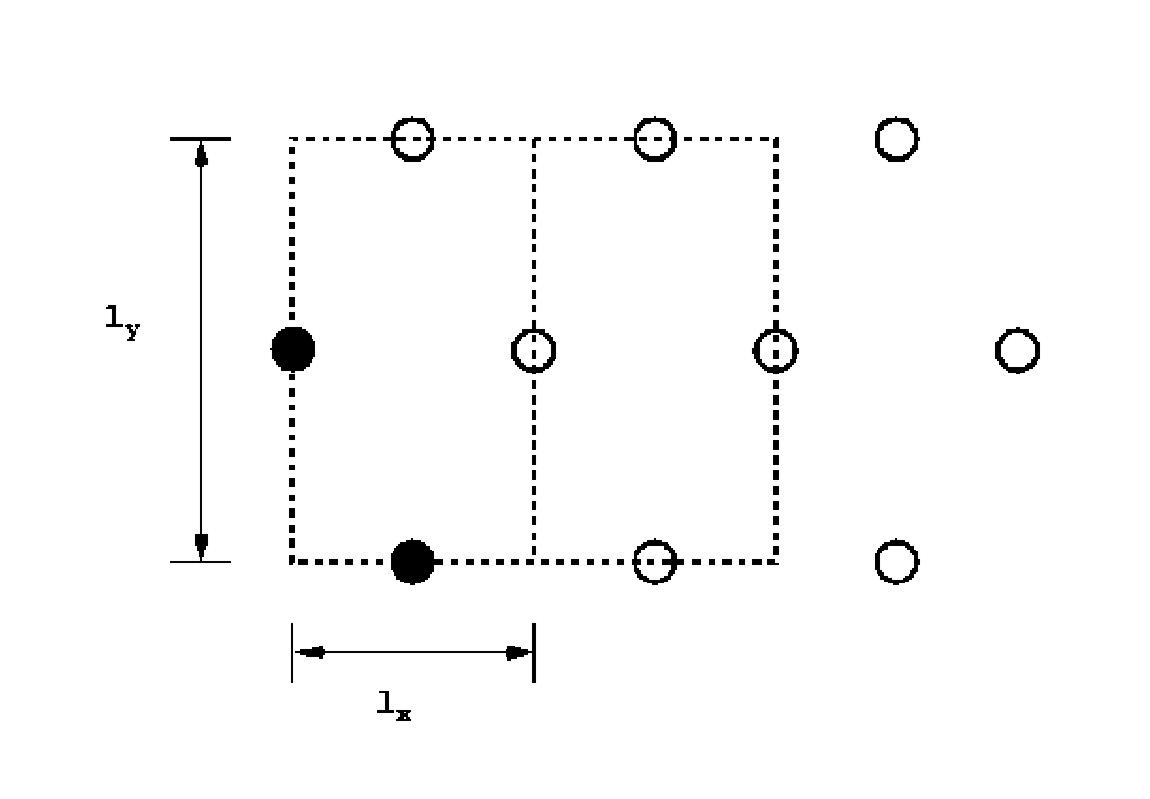
Figure 1.6:
For a particle $i$ in the shaded subcell, eligible
interaction partners $j$ can be only from the subcells marked with
a dot
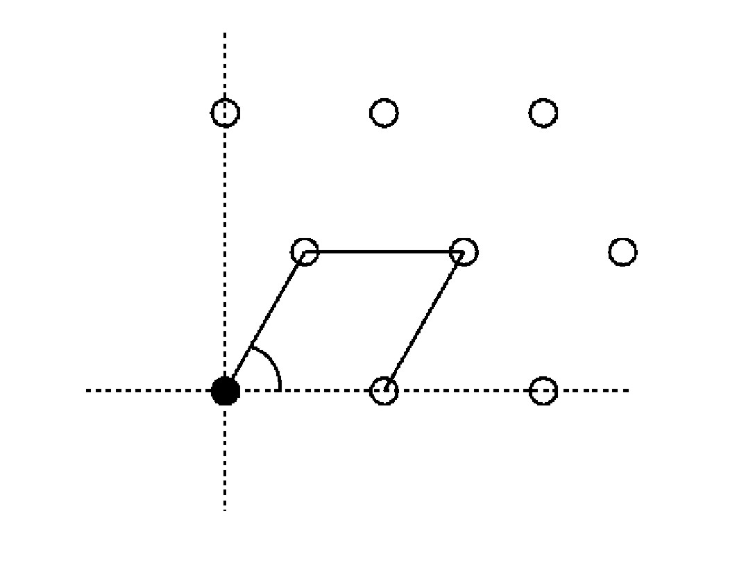
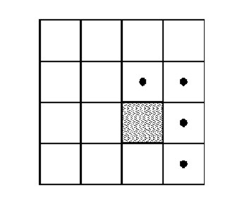
Figure 1.7:
To avoid duplication of pair property calculations, only the
marked cells should be scanned for partners of a particle in the shaded
cell. (But respect periodic b.c.!)
The following description follows the discussion found in Hockney's
book [HOCKNEY, EASTWOOD: COMPUTER SIMULATION USING PARTICLES.
McGraw-Hill, New York 1981].
Define two pointer arrays defined as follows:
$hoc[k= 1 \dots M^{3}]$ (for "head of chain"); its
$k$-element contains the largest particle number of all inhabitants of
cell $k$.
$ll[i=1 \dots N]$
( "linked list"); number of the next (i.e. lower)
particle in the presently treated cell; when $ll[i]=0$ that cell is finished.
Procedure:
In a language-free (but Fortran-like) form, proceed as follows:
	do 100 k=1,ncell // where usually ncell=M^3
100	hoc(k)=0
	do 200 i=1,n
	  icell=1+int(x(i)/cl)  //where cl=l=L/M
	         +int(y(i)/cl)*M
		 +int(z(i)/cl)*M*M
	  ll(i)=hoc(icell)
	  hoc(icell)=i
200	continue
These few quick steps may be performed at each MD or MC step to update
the linked-cell pointer arrays. When it comes to calculating interactions,
these arrays provide the information about possible partner molecules.
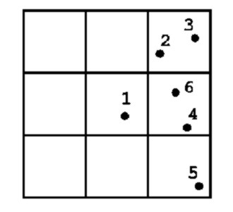
For clarity, consider this example:
Figure 1.8:
See text. Note that the cells are numbered from lower left (1)
to upper right(9)
Later, when it comes to scan the lists (force or energy calculation),
we proceed thus:
For a particle (no. $1$) in cell $5$, we have to scan cells
$3,(5),6,(8),9$ where the brackets denote those cells which in our
example are empty of partners.
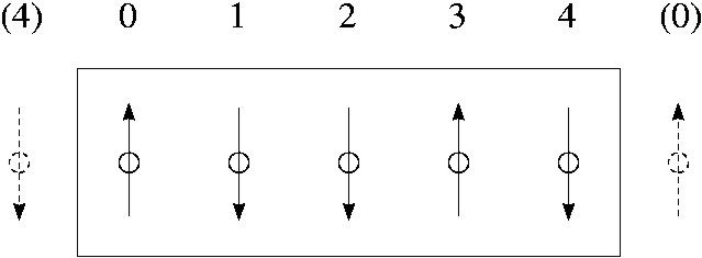
PROJECT MC/MD:
As a first reusable module for a simulation program, write a code to
set up a cubic box of side length $L$ inhabited by up to $N=4 m^{3}$
particles in a face-centered cubic arrangement. Use your favourite programming language
and make the code flexible enough to allow for easy change of volume
(i.e. density). Make sure that the lengths are measured in units of
$\sigma_{LJ}$. For later reference, let us call this subroutine
STARTCONF.
Advice: It is convenient to count the lower, left and front
face of the cube as belonging to the basic cell, while the three other
faces belong to the next periodic cells.
To test for correct arragement of the particles, compute the diagnostic
$
S_{0} \equiv \frac{\textstyle 1}{\textstyle 3}\sum_{i=1}^{N} \left[
\cos (4 m \pi x_{i}/L)+\cos (4 m \pi y_{i}/L)+
\cos (4 m \pi z_{i}/L) \right]
$
which is sometimes called "melting factor". For a fcc
configuration it should be equal to $N$ (why?).
By scaling all lengths, adjust the volume such that the reduced number
density becomes $\rho^{*}=0.6$
PROJECT MD:
Augment the subroutine STARTCONF by a procedure that assigns random
velocities to the particles, making sure that the
sum total of each velocity component is zero.
PROJECT MC/MD:
The second subroutine will serve to compute the total potential
energy in the system, assuming a Lennard-Jones interaction and applying
the nearest image convention: