Statistical Physics and Simulation / Molecular Simulation
Course material
Academic years 2001-..
Franz J. Vesely
University of Vienna
franz.vesely@univie.ac.at
Chapter 6 in my web tutorial on
Computational Physics refers to
simulation. Here follows a more extensive treatment which I also
use in a more advanced course on "Statistical Mechanical Simulation".
Molecular simulation in the U of Vienna Physics curriculum
In 1975 I was a postdoc guest of Konrad Singer at Royal Holloway
College. David Adams, then a postdoc himself, showed me how to do MD,
and how to do it elegantly. I am still striving to learn that second
part.
Back in Vienna I started to offer courses on the
basics and the current applications of molecular simulation. In
1978 my textbook "Computerexperimente an Fluessigkeitsmodellen"
(Physik Weinheim, ISBN 3-87664-041-5) appeared. Other colleagues
at the Institute of Experimental Physics, notably Harald Posch
and Martin Neumann, joined me in applying and teaching various aspects
of molecular simulation.
The growing interest of students forced Martin and me to broaden the
content of the courses we offered - the market for molecular simulators
being rather limited. Thus we installed a regular study curriculum in
"Computational Physics",
covering topics that range from the basics
of finite difference calculus to hydrodynamic and quantum calculations.
Every other year a special course on molecular simulation is offered.
In 1993 I published the German version of a textbook on CompPhys,
and the first English edition appeared in 1994; The current version
of
"Computational Physics - An Introduction", Kluwer-Plenum,
ISBN 0-306-46631-7) is from 2001.
Martin Neumann and I alternate in teaching the CompPhys course which
comprises 3 weekly lectures and 2 hours of workshop, spanning one
full academic year. In the subsequent year students may attend an
Advanced Workshop preparing them for their Master's thesis in CompPhys.
A little history
- 1952, Metropolis, Rosenbluth, Teller: Monte Carlo on 32 Hard disks
- 1957, Alder: Molecular Dynamics of hard spheres; microscopic vortices!
- 1964, Rahman, Verlet: Lennard Jones fluid
- 1968-70, Hoover, Ree: Melting transition for hard disks and hard spheres, then
for soft (LJ) spheres!
- 1970: Harvest time for Liquid State Physics; more complex fluids, too (water,
polymers, ...)
Intramolecular bonds, if
$kT$ is comparable to the bond energy
Born-Huggins-Mayer
$u(r)=
\frac{\textstyle{q_{1}q_{2}}}{\textstyle{4\pi \epsilon_{0}r}}
+ B e^{\textstyle{-\alpha r}} -
\frac{\textstyle{C}}{\textstyle{r^{6}}}-
\frac{\textstyle{D}}{\textstyle{r^{8}}}$
Ionic melts;
$q_{i}$ are the ion charges
Table 1.2:
Anisotropic model potentials in statistical-mechanical simulation:
$u(12)=u(r_{12}, e_{1}, e_{2})$
Hard dumbbells,
hard spherocylinders, etc.
$u(12)= \infty \;\;$
if overlap
$= 0 \;\;\;$
otherwise
First approximation to rigid molecules
Interaction site models, rigid
$u(12)=$ sum of isotropic pair energies
$\textstyle{u(r_{i(1),j(2)})}$,
where several interaction sites $i$ and $j$
are in fixed positions on molecules $1$ and $2$, respectively
Rigid molecules
Interaction site models with non-rigid bonds
$u(12)=$
sum of isotropic pair energies, both intra- and intermolecular
Non-rigid molecules
Kramers-type
$u(12)=$
sum of isotropic pair energies, exclusively between sites on different
molecules; certain intramolecular distances (bonds) and/or angles
are fixed
Flexible molecules, from ethane to biopolymers
Stockmayer
$u(12)=$
Lennard-Jones + point dipoles
First approximation to small polar molecules
Anisotropic Kihara
$u(12)=
4 \epsilon \left[ \left(
\frac{\textstyle{\rho_{12}}}{\textstyle{\sigma}}\right)^{-12}
- \left(
\frac{\textstyle{\rho_{12}}}{\textstyle{\sigma}}\right)^{-6} \right]$
where $\rho_{12}$ is the shortest distance between two linear rods
Rigid linear molecules
with distributed
Lennard-Jones interaction
Gay-Berne
$u(12)=$
$4 \epsilon(12)
\left[ \left(
\frac{\textstyle{r_{12}-\sigma(12)+\sigma_{0}}}{\textstyle{\sigma_{0}}}\right)^{-12}
\right.$
$- \left. \left(
\frac{\textstyle{r_{12}-\sigma(12)+\sigma_{0}}}{\textstyle{\sigma_{0}}}\right)^{-6} \right]$
where $\sigma(12)$ and $\epsilon(12)$ depend on $r_{12}, e_{1}, e_{2}$
and certain substance-specific shape parameters
Liquid crystal molecules of ellipsoidal shape, with
smoothly distributed Lennard-Jones sites
At time $t$, combine the position vectors of the
$N$ atoms into a vector $\Gamma_{c}\equiv$ $\{ r_{1} \dots$
$ r_{N}\}$.
The set of all possible such vectors spans the
$3N$-dimensional "configuration space" $\Gamma_{c}$.
Let $a(\Gamma_{c})$ be some property of the
$N$-body system, depending on the positions of all particles
(i.e. of the microstate $\Gamma_{c}$.)
The thermodynamic average of $a$ is given by
Problem: the probability density $p(\Gamma_{c})$
is known only up to an indetermined normalizing factor.
Thus, $p_{can}(\Gamma_{c})$ $\propto exp[-E(\Gamma_{c})/kT]$,
but the normalizing denominator $Q$ (the Configurational Partition
Function) in
Basic model of ferromagnetic solids:
atoms are fixed on the vertices of a lattice. Their
dipole vectors (spins) may have varying directions: either
up/down (Ising model) or any direction (Heisenberg model).
Microscopic configuration $\Gamma_{c}$: given by
the $N$ spins on the lattice.
Example:
Two-dimensional square Ising lattice; only the four nearest spins
contribute to the energy of spin $\sigma_{i}$
($= \pm 1$). (Three dimensions: six nearest neighbors).
The total energy is
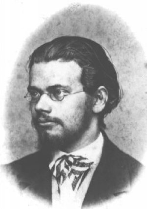 Ludwig Boltzmann would have loved simulation!