| Franz J. Vesely > Lennard-Jones Lines |
Lennard-Jones Lines (LJL)Franz J. Veselyfranz.vesely@univie.ac.at Computational Physics Group, University of Vienna, Boltzmanngasse 5, A-1090 Vienna To JCP paper To Lecture Notes Consider two lines of finite length $L$ containing a homogeneous density of LJ centers. Let $\vec{e}_{1,2}$ be the direction vectors, $\vec{r}_{12}$ the vector between the centers of the two line segments, and $\lambda, \, \mu$ parameters giving the positions of the interacting points along $1$ and $2$. The squared distance between any two such points is given by $r^{2}= \left| r_{12}+\mu \cdot \vec{e}_{2}-\lambda \cdot \vec{e}_{1} \right|^{2} $. The total interaction energy between the two lines is then
$
u(1,2) \equiv u(\vec{r}_{12},\vec{e}_{1},\vec{e}_{2}) =
\frac{\textstyle 1}{\textstyle L^{2}}
\int \limits_{\textstyle 1}d\lambda \int \limits_{\textstyle 2}d\mu \, \,
u_{LJ}\left[ r(\lambda,\mu) \right]
$
with $u_{LJ}(r)=4 \,(r^{-12}-r^{-6})$. We define the triple Gaussian approximation function as $ g_{3G}(r)=\sum_{i=1}^{3}A_{i} \exp\{-B_{i} r^{2}\} $ and demand that it equals $u_{LJ}(r)$ at the points $r=0.7; 0.8; 0.9; 1.0; r_{min}; 1.6$, where $r_{min}=1.12246$ is the minimum point of the LJ potential. The six parameters are then given by
$A(i)=\{
3.9710294335e+05; \; 7.1326116569e+03; \; -5.9236223976e+00
\}
$
and $B(i)=\{ 1.6202936970e+01; \; 8.3948109130e+00; \; 1.2789514461e+00 \} $ 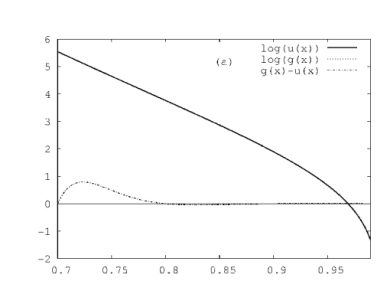
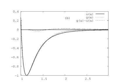
Figure 1: The LJ potential approximated by a sum of three Gaussians: (a) logarithm of $u_{LJ}(r)$ and $g_{3G}(r)$ in the range $r=0.7 - 0.99$; (b) $u(r)$ and $g_{3G}(r)$, range $r= 0.99 - 3$. Solid line: $u_{LJ}$; dashed: $g_{3G}$; the dashed-dot lines denote the deviation $g_{3G}-u_{LJ}$. In place of $\lambda, \mu$ we introduce new parameters $\gamma, \delta $ along the two carrier lines, such that $\gamma = \delta = 0$ at the points of least line-line distance $r_{0}$. The squared distance between two points along the line segments is then
$r^{2}=r_{0}^{2}+\gamma^{2}+\delta^{2}-2 \gamma \delta d$,
with $d = \vec{e}_{1} \cdot \vec{e}_{2}$. Thus each of the three Gauss terms contributes
$
G_{i}=C_{i} \int \limits_{\gamma_{a}}^{\gamma_{b}} d \gamma
\int \limits_{\delta_{a}}^{\delta_{b}} d \delta \,
\exp \left\{ - B_{i} \left(
\gamma^{2}+\delta^{2}-2 \gamma \delta d \right)
\right\}
$
with $C_{i} \equiv A_{i}\exp\{-B_{i} r_{0}^{2} \}$. This is the integral of a bivariate Gaussian over a rectangular region. It can be decomposed into a linear combination of four quadrant integrals: $G_{i}= H_{i}(b,b,d)-H_{i}(a,b,d)-H_{i}(b,a,d)+H_{i}(a,a,d) $, where
$
H_{i}(a,b,d) \equiv C_{i} \,
\int \limits_{\textstyle - \infty}^{\textstyle \gamma_{a}} d \gamma
\int \limits_{\textstyle - \infty}^{\textstyle \delta_{b}} d \delta \,
\exp \left\{
- B_{i} \left( \gamma^{2}+\delta^{2}-2 \gamma \delta d \right)
\right\}
$
etc. Now consider the bivariate normal distribution with density
$
n_{2}(x,y,\rho) \equiv \frac{\textstyle 1}{\textstyle 2 \pi \sqrt{1-\rho^{2}}}
\exp \left\{ - \left( x^{2}+y^{2}-2 x y \rho \right)
/ \left( 2 (1-\rho^{2})\right) \right\}
$
and the cumulative probability
$
N_{2}(a,b,\rho) \equiv
\int \limits_{\textstyle - \infty}^{\textstyle a} d x
\int \limits_{- \infty}^{b} dy \; n_{2}(x,y,\rho)
$
Comparing this standard distribution to our expressions for the $H_(i)$ we find that
$
H_{i}(a,b,d)= \frac{\textstyle C_{i} \pi}{\textstyle B_{i} \sqrt{1-d^{2}}} \,
N_{2} \left(
\gamma_{a}\sqrt{2B_{i}(1-d^{2})}, \delta_{b}\sqrt{2B_{i}(1-d^{2})}, d
\right)
$
etc.
Putting it all together, we have for the potential between two LJ line segments
$
u(\vec{r}_{12},\vec{e}_{1},\vec{e}_{2}) =
\frac{\textstyle 1}{\textstyle L^{2}}
\sum \limits_{i=1}^{3} \left[H_{i}(b,b,d)-H_{i}(a,b,d)-H_{i}(b,a,d)+H_{i}(a,a,d) \right]
$
where the functions $H_{i}$ are as defined before. Thus we have to find an efficient way of evaluating $N_{2}(x,y,\rho)$. Two series expansions, "tetrachoric" and Vasicek's "alternative" series:
Number of terms? -- in most circumstances the series may be truncated at $m=1$ to $8$, with an absolute energy error below $10^{-6}$. Computing times? -- A comparison of computing times is given in Table 1. $m=5$ was used in both configurations, tee and end-to-end.
Computing times (seconds) per pair interaction, for various models. (Pentium M CPU; 1.7 GHz; F77 compiler.) The "tee" configuration corresponds to zero correlation in the bivariate Gaussian representation, while an almost parallel (e.g. end-to-end) configuration relates to $\rho \rightarrow 1$ and thus requires the use of a Vasicek series; see text. For comparison, the potential between two 6-LJ-sites particles as well as the Gay-Berne potential are computed. Compare with other models: In the figure the LJL interaction is compared to multisite potentials with $9 \dots 72$ LJ sites; "tee" configuration; axis length $L=4$; total "LJ load" $Q=1$. 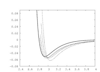
Figure 2: The LJL model as the limiting case of multi-LJ-sites potentials. "tee" position; length of axis: $L=4$. Solid line: LJL; dashed: 9LJ; remaining graphs, approaching LJL: $n=18, 36$ and $72$. 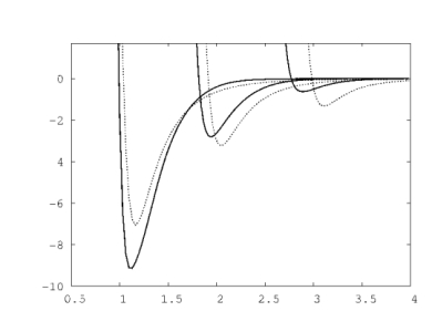
Figure 3: Comparison of the LJ lines (LJL) model with the four-LJ-sites (4LJ) potential with axis length $L=2$. Curves at left: side-by-side configuration with $d \equiv \vec{e}_{1} \cdot \vec{e}_{2}=0.99$; middle: tee configuration; right: end-to-end with $d$ as in side-by-side. Solid lines: LJL potential, dashed: 4LJ potential. Pair Force: The pair force $F_{12}$ acting from 2 on 1 is given by:
Pair Torque: [under construction] The torque $T_{12}$ exerted by 2 on 1 is given by
$
\vec{T}_{12}
= - \vec{e}_{1} \times \nabla_{\textstyle e_{1}} u(1,2)
$
where $ \nabla_{\textstyle e_{1}} \equiv \left\{ \partial / \partial e_{1}^{\alpha} \right\} $ is the derivative with respect to the direction vector $\vec{e}_{1}$. To the best of my knowledge at this date (Sep-07) this derivative has the following form:
Remarks regarding perturbation theory: Hard-body correlate: hard spherocylinder model? Danger: do NOT divide the elementary interaction in the definition of the LJL potential according to WCA, using just the repulsive part of the LJ potential to define the reference interaction. The attractive part is important as it compensates part of the repulsion. Example: $L=4$; end-to-end configuration with distance $r=0.7$ has a considerable probability in the full LJL system but not in the purely repulsive case. Thus the assumption of identical structure in the reference and target systems is not met. The hard body correlate must be found in another way. Any ideas? |