Back to WEBLOG
Shortest Distance between two Line Segments
Franz J. Vesely
May 2002
Model systems made of sticks play a role both in Statistical Mechanics
(Hard Spherocylinders, Linear Kihara Molecules) and in Robotics (Robot
Arms). The basic exercise in both settings is to determine the shortest
distance between two such line segments. The method sketched here was
described by Allen et al., Adv. Chem. Phys. Vol. LXXXVI, 1993, p.1.
Shortest distance between two line segments
We divide the problem in two steps:
- Determine the distance
 in 3D space between
the two ``carrier'' lines of the line segments; keep the vector
in 3D space between
the two ``carrier'' lines of the line segments; keep the vector
 between the closest points
  on the two lines.
Note that this vector is normal to both lines.
on the two lines.
Note that this vector is normal to both lines.
- Project the two lines onto a plane normal to .
Since is normal to both lines this projection conserves
distances on the lines.
Now determine the shortest distance
 within the plane between
the two line segments.
within the plane between
the two line segments.
The shortest total distance is then
 .
.
Distance between two lines in 3D:
Let  and
and  denote the center positions and
directional unit vectors of the two segments of lengths
denote the center positions and
directional unit vectors of the two segments of lengths  .
The carrier lines
.
The carrier lines  are then given by
 and
and
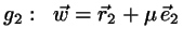 .
The vector between any two points on the two lines is then
.
The vector between any two points on the two lines is then
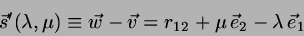 |
(1) |
with
 . The shortest among these
vectors is perpendicular to both lines; thus
. The shortest among these
vectors is perpendicular to both lines; thus
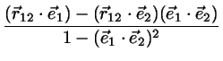
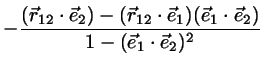
Solving for the line parameters we find
(If you suspect that your lines may be nearly parallel, you should take
care of the small denominator in some meaningful manner.)
The vector between the proximate points is
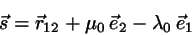 |
(6) |
and the minimum interline distance is
 .
.
Distance between two line segments in 2D:
Think of the two carrier lines being projected down into a plane
normal to . This projection, being normal to both lines,
conserves distances along the lines.
The intersection point is, of course, given by
 .
Taking this as the origin, the lines are now represented
by
.
Taking this as the origin, the lines are now represented
by
 and
and
 .
For points on the given segments the parameters
.
For points on the given segments the parameters  and
and  are confined to
 and
and
 which defines a
rectangle in (
which defines a
rectangle in (
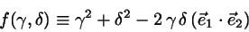
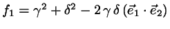
 ) parameter space. We are now searching
for the minimum of
) parameter space. We are now searching
for the minimum of
 within that parameter region:
![$\vert r_{in} \vert^{2} = \min \left[f(\gamma,\delta)\right]$](img33.png) with
with
 |
(7) |
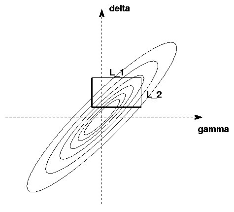
Figure: Finding the minimum of f=gamma**2+delta**2+2*gamma*delta*(e1*e2).
The bold sides of the rectangle are the lines gamma_m, delta_m (see text)
If the origin is contained in the rectangle,
life is easy: the origin is the minimum, and
the in-plane distance is zero!
If not, proceed as follows:
First, find the lines  ,
,  that are nearest to the
origin:
that are nearest to the
origin:
 ,
,
 .
.
Now choose the line
 and find the value of that
minimizes
and find the value of that
minimizes  :
:
 .
If
.
If  is in the permitted range, we set
 ;
otherwise, we pick the allowed nearest to .
The distance at
is computed:
;
otherwise, we pick the allowed nearest to .
The distance at
is computed:
The same steps are taken for
 and its optimal ,
yielding a trial value
and its optimal ,
yielding a trial value  .
.
With
 we complete the calculation of the
shortest total distance,
we complete the calculation of the
shortest total distance,
 |
(8) |
Here is a skeleton code that does the job:
	subroutine overlap(i,j)

! Given two line segments in space, with center positions r1,r2,
! direction vectors e1,e2 and segment lengths L1,L2, calculate the
! shortest distance between the two segments

	implicit double precision (a-h,o-z)
	common side
	common /configuration/x(2),y(2),z(2),ex(2),ey(2)
     1	,ez(2),xlen(2)

! See Allen, Evans, Frenkel, Mulder, Adv. Chem. Phys. Vol. LXXXVI, p. 1

! r1:
	x1=x(i)
	y1=y(i)
	z1=z(i)
! r2:
	x2=x(j)
	y2=y(j)
	z2=z(j)
! distance vector between centers:
	x12=x2-x1
	y12=y2-y1
	z12=z2-z1
! In MC/MD it may be appropriate here to apply the nearest image
! convention:
	if (x12.lt.-side/2.) x12=x12+side
	if (x12.ge.side/2.) x12=x12-side
	if (y12.lt.-side/2.) y12=y12+side
	if (y12.ge.side/2.) y12=y12-side
	if (z12.lt.-side/2.) z12=z12+side
	if (z12.ge.side/2.) z12=z12-side

! e1:
	ex1=ex(i)
	ey1=ey(i)
	ez1=ez(i)
! e2:
	ex2=ex(j)
	ey2=ey(j)
	ez2=ez(j)

! First, find the normal vector en at minimal distance between the
! carrier lines g1 and g2:
! Since en is normal both to e1 and e2 we have for any normal vector
!
! r12*e1=lam-mu*(e1*e2)
! r12*e2=lam*(e1*e2)-mu

! which yields (excluding the case e1*e2=0)

! lam0=[(e1*r12)-(e1*e2)(e2*r12)]/[1-(e1*e2)^2]
! mu0=-[(e2*r12)-(e1*e2)(e1*r12)]/[1-(e1*e2)^2]
!
	e1r=ex1*x12+ey1*y12+ez1*z12
	e2r=ex2*x12+ey2*y12+ez2*z12
	e12=ex1*ex2+ey1*ey2+ez1*ez2
	recipr=1./(1.-e12*e12)
	xla0=recipr*(e1r-e12*e2r)
	xmu0=-recipr*(e2r-e12*e1r)

! Shortest perpendicular distance between carrier lines:
	xx12=x12+xmu0*ex2-xla0*ex1
	yy12=y12+xmu0*ey2-xla0*ey1
	zz12=z12+xmu0*ez2-xla0*ez1
	rnsq=xx12*xx12+yy12*yy12+zz12*zz12
	dd=sqrt(rnsq)


! Now for the squared in-plane distance risq between two line segments:

! Rectangle half lengths h1=L1/2, h2=L2/2
	xlen1=xlen(i)
	xlen2=xlen(j)
	h1=0.5*xlen1
	h2=0.5*xlen2

! If the origin is contained in the rectangle,
! life is easy: the origin is the minimum, and
! the in-plane distance is zero!

	if ((xla0*xla0.le.h1*h1).and.(xmu0*xmu0.le.h2*h2)) then
	  risq=0. 	! Simple overlap

	else
! Find minimum of f=gamma^2+delta^2-2*gamma*delta*(e1*e2)
! where gamma, delta are the line parameters reckoned from the intersection
! (=lam0,mu0)


! First, find the lines gamm and delm that are nearest to the origin:
	  gam1=-xla0-h1
	  gam2=-xla0+h1
	  gamm=gam1
	  if (gam1*gam1.gt.gam2*gam2) gamm=gam2
	  del1=-xmu0-h2
	  del2=-xmu0+h2
	  delm=del1
	  if (del1*del1.gt.del2*del2) delm=del2

! Now choose the line gamma=gamm and optimize delta:
	  gam=gamm
	  delms=gam*e12
	  aa=xmu0+delms	! look if delms is within [-xmu0+/-L/2]:
	  if (aa*aa.le.h2*h2) then
	    del=delms		! somewhere along the side gam=gamm
	  else
! delms out of range --> corner next to delms!
	    del=del1
	    a1=delms-del1
	    a2=delms-del2
	    if (a1*a1.gt.a2*a2) del=del2
	  endif
! Distance at these gam, del:
	  f1=gam*gam+del*del-2.*gam*del*e12

! Now choose the line delta=deltam and optimize gamma:
	  del=delm
	  gamms=del*e12
	  aa=xla0+gamms	! look if gamms is within [-xla0+/-L/2]:
	  if (aa*aa.le.h1*h1) then
	    gam=gamms		! somewhere along the side gam=gamm
	  else
! gamms out of range --> corner next to gamms!
	    gam=gam1
	    a1=gamms-gam1
	    a2=gamms-gam2
	    if (a1*a1.gt.a2*a2) gam=gam2
	  endif
! Distance at these gam, del:
	  f2=gam*gam+del*del-2.*gam*del*e12

! Compare f1 and f2 to find risq:
	  risq=f1
	  if(f2.lt.f1) risq=f2
	endif

! Distance of closest approach squared =
! in-plane distance squared + normal distance squared:
	rclsq=rnsq+risq
	rcl=sqrt(rclsq)

	return
	end
F. J. Vesely / University of Vienna