| Franz J. Vesely > CompPhys Tutorial > Exercises and Projects |
Exercises and ProjectsE1: Harmonic Oscillator (Ch.1 Sec. 4) a) Write a program to tabulate and/or draw the analytical solution to the HO equation. (You may achieve a very concise visualization by displaying the trajectory in phase space, i.e. in the coordinate system $\{ x; \dot{x} \}$; where for $\dot{x}$ the approximation $\dot{x} \approx (x_{n+1}-x_{n-1})/2 \Delta t$ may be used.) Choose values of $\omega_{0}^{2}$, $\Delta t$ and $x_{0}, \dot{x}_{0}$, and use these to determine the exact value of $x_{1}$. Starting with $x_{0}$ and $x_{1}$, employ the above algorithm to compute the further path $\{x_{n} ; n=2,3,\dots \}$. Test the performance of your program by varying $\Delta t$ and $\omega_{0}^{2}$. b) Now apply your code to the anharmonic oscillator
\frac{\textstyle d^{2}x}{\textstyle dt^{2}} = - \omega_{0}^{2} x - \beta x^{3}
To start the algorithm you may use the approximate value given by
x_{1} \approx x_{0} + \dot{x}_{0} \Delta t + \ddot{x}_{0}
\frac{\textstyle (\Delta t)^{2}}{\textstyle 2}
c) The planar pendulum is described by the equation of motion
\frac{\textstyle d^{2}\phi}{\textstyle dt^{2}} =
- \frac{\textstyle g}{\textstyle l} sin \phi
Solution strategies vary between the three regions: $\phi$ very small; $\phi$ small; $\phi$ arbitrary. Very small $\phi$: Here $\sin \phi \approx \phi$, and the e.o.m. is that of a harmonic oscillator, with the usual analytic solution. Small $\phi$: We may put $\sin \phi \approx \phi - \phi^{3}/6$, adding an anharmonic term to the e.o.m. Again, an analytical solution may be found, but it is more involved than in the harmonic case; see Landau-Lifshitz, Mechanics. Any $\phi$: The exact solution is known in implicit form:
t(\phi) =
\int \limits_{0}^{\phi}
\frac{\textstyle d \phi'}{\textstyle
\sqrt{\textstyle (2/ml^{2}) \left[E+mgl \cos \phi' \right]}}
One may clumsily invert this equation for regular times $t_{k}$, using Newton-Raphson. Instead, one may choose to simulate the pendulum, using the Stoermer-Verlet algorithm:
\phi(t_{n+1}) =
2 \phi(t_{n})-\phi(t_{n-1})-\frac{\textstyle g}{\textstyle l} \sin \phi(t_{n})
(\Delta t)^{2}
As a starting value for $\phi(t_{1})$ one may use the Taylor approximation
\begin{eqnarray}
\phi_{1} &\approx& \phi_{0} + \dot{\phi}_{0} \Delta t + \ddot{\phi}_{0}
\frac{\textstyle (\Delta t)^{2}}{\textstyle 2}
\end{eqnarray}
E2: Thermal Conduction (Ch.1 Sec. 4)
\begin{eqnarray}
\frac{\textstyle \partial T(x,t)}{\textstyle \partial t} & = &
\lambda \frac{\textstyle \partial^{2} T(x,t)}{\textstyle \partial x^{2}}
\end{eqnarray}
Writing $T_{i}^{n} \equiv T(x_{i},t_{n}) $,
we arrive at the "FTCS scheme" ("forward-time, centered-space")
$
\begin{eqnarray}
\frac{\textstyle 1}{\textstyle \Delta t}[T_{i}^{n+1}-T_{i}^{n}] & \approx &
\frac{\textstyle \lambda}{\textstyle (\Delta x)^{2}}
[T_{i+1}^{n}-2 T_{i}^{n}+T_{i-1}^{n}]
\end{eqnarray}
$
or
\begin{eqnarray}
T_{i}^{n+1}&=&(1-2a) T_{i}^{n} + a(T_{i-1}^{n}+T_{i+1}^{n}) \; ,
\;\;\;
with
\;\;\;
a &\equiv& \lambda \Delta t/(\Delta x)^{2}
\end{eqnarray}
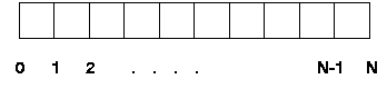
for $i=1, \dots N-1$ (and $T_{0}^{n+1}$, $T_{N}^{n+1}$ given as boundary conditions). Now let us divide the rod into $N=10$ pieces of equal length, with node points $i=0,\dots N$, and assume the boundary conditions $T(0,t) \equiv T_{0}^{n}=1.0$ and $T(L,t) \equiv T_{10}^{n}=0.5$. The values for the temperature at time $t=0$ (the initial values) are $T_{1}^{0}=T_{2}^{0}=$ $ \dots T_{5}^{0}= 1.0$ and $T_{6}^{0}=T_{7}^{0}=$ $ \dots T_{9}^{0}= 0.5$ (step function). E3: Thermal Conduction Revisited (Ch.2 Sec. 5) We will need the Recursion Method of Sec. 2.2.4 for solving $A \cdot x = b$. Therefore, as a warm-up exercise, it may help to write a code to reproduce the Example given there, with
$
A =
\left( \begin{array}{cccc}
2 & 1 & 0 & 0 \\
2 & 3 & 1 & 0 \\
0 & 1 & 4 & 2 \\
0 & 0 & 1 & 3
\end{array} \right)
\;\; \;\; {\rm and} \;\;\; b =
\left( \begin{array}{c} 1 \\2 \\3 \\4 \end{array} \right)
$
Now redo the earlier exercise on One-dimensional thermal conduction by applying the implicit scheme in place of the FTCS method. The equation to be solved is the "implicit scheme of first order"
$
\begin{eqnarray}
&&
\frac{\textstyle 1}{\textstyle \Delta t} [T_{i}^{n+1}-T_{i}^{n}]
=\frac{\textstyle \lambda}{\textstyle (\Delta x)^{2}}
[T_{i+1}^{n+1}-2T_{i}^{n+1}+T_{i-1}^{n+1}]
\end{eqnarray}
$
which may be written, using $a \equiv \lambda\Delta t/(\Delta x)^{2}$,
$
\begin{eqnarray}
&&
A \cdot T^{n+1} = T^{n}
\end{eqnarray}
$
where (for fixed $T_{0}$ and $T_{N}$)
$
\begin{eqnarray}
&&
A \equiv
\left(
\begin{array}{cccccc}
1 & 0 & 0 & . & . & 0 \\
- a & 1+2a & -a & 0 & . & 0 \\
0 & . & . & . & 0 & . \\
. & . & . & . & . & . \\
. & . & . & 0 & 0 & 1
\end{array}
\right)
\end{eqnarray}
$
This tridiagonal system may be solved by the Recursion Method. Use various values of $\Delta t$ (and therefore $a$.) Compare the efficiencies and stabilities of the two methods. E4: Transformation method (Ch.3 Sec. 2) (a) Warm-up (no coding): A powder of approximately spherical metallic grains is used for sintering. The diameters of the grains obey a normal distribution with $\langle d \rangle =2 \mu m$ and $\sigma=0.25 \mu m$. Calculate the distribution of the grain volumes. (b) Lorentzian density: Write a codelet which produces random variates with probability density
$
p(x) = \frac{\textstyle 1}{\textstyle\pi} \frac{\textstyle 1}{\textstyle 1+x^{2}}
\;\;\;{\rm (Lorentzian),} \;\;\;\;
x \epsilon (\pm \infty)
$
using the transformation method. Plot a frequency histogram of the produced random numbers and compare it with the given $p(x)$. Also, plot the distribution function $P(x)$ pertaining to the given density. E5: Bivariate Gaussian generator (Ch.3 Sec. 2) We want to construct a generator that produces pairs of random numbers $\vec{x} \equiv (x_{1},x_{2})$ having a joint density $p(x_{1},x_{2})$ that is bivariate Gaussian with correlation matrix
$
S \equiv \left\{ < x_{i} x_{j} > \right\}
= \left( \begin{array}{cc}3 & 2\\ \\2 & 4\end{array} \right)
$
(a) Redo the calculation of the diagonalization matrix $T$, either by hand or in a program. (b) Write a code that uses this matrix $T$ to generate a sequence of random vectors $\vec{x}$ with the given properties. Determine the actual statistics $\langle x_{1}^{2}\rangle$, $\langle x_{2}^{2}\rangle$ and $\langle x_{1}x_{2}\rangle$ to see if they indeed approach the given values of $3$, $4$, and $2$. (c) Extra point: If you feel up to it, generalize your code to trivariate Gaussian random numbers. E6: Markov sequence (Ch.3 Sec. 3) We wish to produce a stationary Gaussian Markov sequence $\{x(n);\;n=0,\dots\}$ with autocorrelation function $ \langle x(n)x(n+k) \rangle = (A / 2 \beta) e^{-\beta k\Delta t} $ where the values of $A$, $\beta$ and $\Delta t$ are given. Employ the "Langevin Shuffle" procedure described in the text. Check if the sequence shows the expected autocorrelation. E7: Wiener Lévy Process (Ch.3 Sec. 3) 500 random walkers set out from positions $\{ x(0)_{i}, i=1 \dots 500 \}$ homogeneously distributed in the interval $[-1,1]$. The initial particle density is thus rectangular. Each of the random walkers is now set on its course to perform its own one-dimensional trajectory, with $A\Delta t= 0.01$. Sketch the particle density after 100, 200, ... steps. E8: Metropolis rule (Ch.3 Sec. 3) Let $p(x)=A \, \exp[-x^{2}]$ be a desired probability density. Apply the Metropolis prescription to generate a Markov chain of random numbers with this density. Confirm that the autocorrelation is not zero: $\langle x(n)x(n+k) \rangle \neq 0$. E9: Simulated Annealing (Ch.3 Sec. 4) Create (yes, fake!) a table of "measured values with errors" according to
$
y_{i}=f(x_{i};c_{1},\dots c_{6})+\xi_{i},\;\;\; i=1,20
$
with $\xi_{i}$ coming from a Gauss distribution with suitable variance, and with the function $f$ defined by
$
f(x;c)\equiv c_{1}e^{\textstyle - c_{2}(x-c_{3})^{2}}
+c_{4}e^{\textstyle - c_{5}(x-c_{6})^{2}}
$
($c_{1} \dots c_{6}$ being a set of arbitrary coefficients).
Using these data, try to reconstruct the parameters $c_{1}\dots c_{6}$ by fitting the theoretical function $f$ to the table points $(x_{i},y_{i})$. The cost function is
$
U(c)\equiv \sum \limits_{i}\left[ y_{i}-f(x_{i};c)\right]^{2}
$
Choose an initial vector $c^{0}$ and perform an MC random walk through
$ c$-space, slowly lowering the temperature.
E10: Genetic Optimization (Ch.3 Sec. 4) Apply the simple genetic algorithm to find the minimum of the function $[2sin(10x-1)]^{2}+10(x-1)^{2}$ within the interval $[0,2]$. E11: Ordinary Differential Equations / Symplectic Algorithms (Ch.4 Sec. 2) Apply the (non-symplectic) RK method and the (symplectic) Størmer-Verlet algorithm (or the Candy procedure) to the one-body Kepler problem with elliptic orbit. Perform long runs to assess the long-time performance of the integrators. (For RK the orbit should eventually spiral down towards the central mass, while the symplectic procedures should only give rise to a gradual precession of the perihelion.) E12: Ordinary Differential Equations / Various Algorithms (Ch.4 Sec. 2) Write a code that permits to solve a given second-order equation of motion by various algorithms. Start by applying it to an analytically solvable problem, such as the harmonic oscillator or the 2-body Kepler problem. Include in your code tests that do not rely on the existence of an analytical solution - for example, energy conservation. Explore the stabilities and accuracies of the diverse techniques. Finally, apply the code to more complex problems such as the anharmonic oscillator or the many-body Kepler problem. The following Projects will generally be treated in the second (summer) term [No number]: Reduced units (Ch.6 Sec. 1) Consider a pair of Lennard-Jones particles with $\epsilon=1.6537 \cdot 10^{-21} J$ and $\sigma=3.405 \cdot 10^{-10} m$ (typical for Argon). Let the two molecules be situated at a distance of $3.2 \cdot10^{-10}m$ from each other. - Calculate the potential energy of this arrangement. - Do the same calculation using $\epsilon$ and $\sigma$ as units of energy and length, respectively. These parameters then vanish from the expression for the pair energy, and the calculation is done with quantities of order $1$. - With the above units for energy and length, together with the atomic mass unit, compute the metric value of the self-consistent unit of time? Let one of the particles have a metric speed $v=500 m/s$, typical of the thermal velocities of atoms or small molecules. What is the value of $v$ in self-consistent units? P1 / Project MC/MD: (Ch.6 Sec. 1) As a first reusable module for a simulation program, write a code to set up a cubic box of side length $L$ inhabited by up to $N =4 m^{3}$ particles in a face-centered cubic arrangement. Use your favourite programming language and make the code flexible enough to allow for easy change of volume (i.e. density). Make sure that the lengths are measured in units of $\sigma_{LJ}$. For later reference, let us call this subroutine STARTCONF. Advice: It is convenient to count the lower, left and front face of the cube as belonging to the basic cell, while the three other faces belong to the next periodic cells.
To test for correct arrangement of the particles, compute the diagnostic
$S_{0} \equiv \frac{1}{3} \sum \limits_{i}^{N} \left[
\cos (4 m \pi x_{i}/L)+\cos (4 m \pi y_{i}/L)+
\cos (4 m \pi z_{i}/L) \right]
$
which is sometimes called "melting factor". For a fcc configuration it should be equal to $N$ (why?). By scaling all lengths, adjust the volume such that the reduced number density becomes $\rho^{*}=0.6$.
Augment the subroutine STARTCONF by a procedure that assigns random
velocities to the particles, making sure that the
sum total of each velocity component is zero.
P2 / Project MC/MD: (Ch.6 Sec. 1) The second subroutine will serve to compute the total potential energy in the system, assuming a Lennard-Jones interaction and applying the nearest image convention:
$
E_{pot}=\frac{1}{2}\sum \limits_{i} \sum \limits_{j \neq i} u_{LJ}(r_{ij})
= \sum \limits_{i}^{N-1} \sum \limits_{j=i+1}^{N} u_{LJ}(r_{ij})
$
Write such a subroutine and call it ENERGY. Use it to compute the energy in the system created by STARTCONF. P3 / Project MC [fluid]: (Ch.6 Sec. 2) Write a subroutine MCSTEP which performs the basic Monte Carlo step as described in Fig. 6.2: selecting at random one of the LJ particles that were placed on a lattice by STARTCONFIG, displace it slightly and apply the PBC; then compute the new potential energy (using NIC!) and check whether the modified configuration is accepted or not, given a specific temperature $T^{*}$; if accepted, the next configuration is the modified one, otherwise the old configuration is retained for another step. Write a main routine to combine the subroutines STARTCONF, ENERGY, and MCSTEP into a working MC program. P4 / Project MC [lattice]: (Ch.6 Sec. 2) Let $N=n.n$ spins $\sigma_{i}= \pm 1; \; i, \dots N$ be situated on the vertices of a two-dimensional square lattice. The interaction energy is defined by
$
E = \sum \limits_{i} E_{i} = -\frac{1}{2} \sum \limits_{i}^{N}
\sum \limits_{j}^{4} \sigma_{i} \sigma_{j}
$
where the sum over $j$ involves the 4 nearest neighbors of spin $i$. Periodic boundary conditions are assumed.
P5 / Project MD [hard disks]: (Ch.6 Sec. 3) For a two-dimensional system of hard disks, write subroutines to a) set up an initial configuration (simplest, though not best: square lattice;) b) calculate $t(i)$ and $j(i)$; c) perform a pair collision. Combine these subroutines into an MD code. To avoid the difficulty mentioned at the end of the preceding figure, one might simply use reflecting boundary conditions, doing a "billiard dynamics" simulation. P6 / Project MD [Lennard-Jones]: (Ch.6 Sec. 3) Augment the subroutine module ENERGY such that it computes, for each Lennard-Jones particle $i$ in the system, the total force exerted on it by all other particles $j$: $ K_{i} \equiv \sum \limits_{j \neq i} K_{ij}$, with $ K_{ij}$ as given above; remember to apply the nearest image convention. Write a subroutine MOVE to integrate the equations of motion by a suitable algorithm such as Verlet's. Having advanced each particle for one time step, do not forget to apply periodic boundary conditions to retain them all in the simulation box. Write a main routine that puts the subroutines STARTCONF, ENERGY and MOVE to work. Test your first MD code by monitoring the mechanically conserved quantities.
Do a number of MD steps - say, $50-100$ - and average the
quantity $| v^{*}|^{2}$ to estimate the actual temperature.
To adjust the temperature to a desired value, scale all
velocity components of all particles in a suitable way. Repeat
this procedure up to 10 times. After $500 - 100$ steps the
fluid will normally be well randomized in space, and the temperature
will be steady - though fluctuating slightly.
P7 / Project MC/MD [Lennard-Jones]: (Ch.6 Sec. 4) In your Lennard-Jones MD and MC programs, include a procedure to calculate averages of the total potential energy and the virial as defined by
$
W\equiv\sum \limits_{i}\vec{K}_{i}\cdot \vec{r}_{i} = -\frac{\textstyle 1}{\textstyle 2}
\sum \limits_{i} \sum \limits_{j} \vec{K}_{ij}\cdot \vec{r}_{ij}
$
From these compute the internal energy and the pressure. Compare with results from literature, e.g. [ MCDONALD 74, VERLET 67]. Allow for deviations in the $5-10\%$ range, as we have omitted a correction for the finite sample size (`cutoff correction'). P8 / Project MC/MD [Lennard-Jones]: (Ch.6 Sec. 4) Augment your Lennard-Jones MD (or MC) program by a routine that computes the pair correlation function $g(r)$ according to the procedure given above; remember to apply the nearest image convention when computing the pair distances. As the subroutine ENERGY already contains a loop over all particle pairs $(i,j)$, it is best to increment the $g(r)$ histogram within that loop.
Plot the PCF and see whether it resembles the one given in
Figure 6.6.
P9 / Project MD [Lennard-Jones]: (Ch.6 Sec. 4)
Exercise: Path Integral MC (Ch.7 Sec. 2) Here is a little stand-alone exercise referring to the PIMC method.
vesely 2006
|