| Franz J. Vesely > CompPhys Tutorial > Selected Applications > Hydrodynamics |
8.1 Compressible Flow without ViscosityExample: Frictionless air flow in the vicinity of an aircraft. The flow equations in Eulerian formulation reduce to
$
\begin{eqnarray}
\frac{\textstyle \partial \rho }{\textstyle \partial t}+ \nabla \cdot \rho \vec{v} &=& 0
\\
\frac{\textstyle \partial \rho \vec{v}}{\textstyle \partial t}+ \nabla \cdot
\left[ \rho \vec{v} \vec{v} \right] + \nabla p &=& 0
\\
\frac{\textstyle \partial e}{\textstyle \partial t}+ \nabla \cdot \left[ (e+p) \vec{v} \right]&=&0
\end{eqnarray} $
(8.5-8.7)
Euler derivative: laboratory-fixed coordinate system; $\partial / \partial t$ at a fixed point in space Lagrange derivative: properties of a volume element that is moving along with the flow; $ d /dt \equiv \partial / \partial t + \vec{v} \cdot \nabla $ $\longrightarrow$ Lagrange form of the flow equations:
$ \begin{eqnarray}
\frac{\textstyle d \rho}{\textstyle dt} &=& - \rho \nabla \cdot \vec{v}
\\
\rho \frac{\textstyle d \vec{v}}{\textstyle dt} &=& - \nabla p
\\
\frac{\textstyle d e}{\textstyle dt} &=& - (e+p) \nabla p
-(\vec{v} \cdot \nabla)\, p
\\
&=& -e (\nabla \cdot \vec{v}) - \nabla \cdot (p \vec{v})
\end{eqnarray} $
(8.8-8.10)
where the last equation may be written (see 8.4),
$
\frac{\textstyle d \epsilon}{\textstyle dt} = - \, \frac{\textstyle p}{\textstyle \rho} \,(\nabla \cdot \vec{v})
$
(8.11)
8.1.1 Explicit Eulerian Methods
Example: 1D Euler / Lax
$ \begin{eqnarray}
\rho_{j}^{n+1}&=&\frac{\textstyle 1}{\textstyle 2}\left(\rho_{j+1}^{n}+\rho_{j-1}^{n} \right)
-\frac{\textstyle \Delta t}{\textstyle 2 \Delta x}
\left(\rho_{j+1}^{n} v_{j+1}^{n}-\rho_{j-1}^{n}v_{j-1}^{n} \right)
\\
\rho_{j}^{n+1}v_{j}^{n+1}&=&\frac{\textstyle 1}{\textstyle 2}
\left(\rho_{j+1}^{n}v_{j+1}^{n}+\rho_{j-1}^{n}v_{j-1}^{n}\right)
-\frac{\textstyle \Delta t}{\textstyle 2 \Delta x}
\left[\rho_{j+1}^{n}(v_{j+1}^{n})^{2}+p_{j+1}^{n}
-\rho_{j-1}^{n}(v_{j-1}^{n})^{2}-p_{j-1}^{n} \right]
\\
e_{j}^{n+1}&=&\frac{\textstyle 1}{\textstyle 2}\left(e_{j+1}^{n}-e_{j-1}^{n} \right)
-\frac{\textstyle \Delta t}{\textstyle 2 \Delta x}
\left[
\left(e_{j+1}^{n}+p_{j+1}^{n}\right)v_{j+1}^{n}
-\left(e_{j-1}^{n}+p_{j-1}^{n}\right)v_{j-1}^{n}
\right]
\end{eqnarray} $
(8.14-8.16)
8.1.2 Particle-in-Cell Method (PIC)Consider an ideal gas; assume adiabatic equation of state (fast flow or slow conduction of heat): $p/\rho^{\gamma}= c$ constant in a flowing element $\longrightarrow$ Lagrangian time derivative $\partial c / \partial t + \vec{v} \cdot \nabla c = 0$. Therefore
$
\frac{\textstyle \partial }{\textstyle \partial t} \left[ \rho c \right]+ \nabla \cdot
\left[ \rho c \vec{v} \right] = 0
$
(8.17)
(continuity equation for $c$).
$\longrightarrow$ Flow equations:
$ \begin{eqnarray}
\frac{\textstyle \partial \rho }{\textstyle \partial t}+ \nabla \cdot \left( \rho \vec{v} \right)
&=& 0
\\
\frac{\textstyle \partial \rho \vec{v}}{\textstyle \partial t}+ \nabla \cdot
\left( \rho \vec{v} \vec{v} \right) &=& -\nabla p
\\
\frac{\textstyle \partial }{\textstyle \partial t} \left( \rho c \right) +
\nabla \cdot \left( \rho c \vec{v} \right) &=& 0
\end{eqnarray} $
(8.18-20)
Strategy:
Here is the procedure in concise form:
Particle-in-cell method. Note that pressure gradients are evaluated using an Eulerian grid, while the transport of mass, momentum and energy is treated in continuous space. 8.1.3 Smoothed Particle Hydrodynamics (SPH)Motivation: PIC technique uses both Eulerian and Lagrangian elements. Average density within a cell = number of point particles in that cell. Can we represent the local fluid density without a grid? Lucy and Gingold & Monaghan: load each particle with a spatially extended interpolation kernel $\longrightarrow$ Average local density = sum over the individual contributions. Let $w(\vec{r}-\vec{r_{i}})$ denote the interpolation kernel centered around $\vec{r_{i}}$. Then the local density at $\vec{r}$ is
$
\langle \rho(\vec{r})\rangle =
\sum \limits_{i=1}^{N} m_{i}\, w(\vec{r}-\vec{r_{i}})
$
(8.33)
Generally, a property $A(\vec{r})$ is represented by its "smoothed particle estimate"
$
\langle A(\vec{r})\rangle =
\sum \limits_{i=1}^{N} m_{i}\,
\frac{\textstyle A(\vec{r}_{i})}{\textstyle \rho(\vec{r}_{i})} \,
w(\vec{r}-\vec{r_{i}})
$
(8.34)
Form of the interpolation kernel: Gaussian or polynomial Example:
$
w(\vec{s}) = \frac{\textstyle 1}{\textstyle \pi^{3/2}d^{3}} \,
e^{\textstyle - s^{2}/d^{2}}
$
(8.35)
with a width $d$ chosen such that the number of particles within $d$ is $N \approx 5$ in 2 dimensions and $N \approx 15$ for 3 dimensions. Now rewrite the Lagrangian equations of motion 8.8-8.11 in smoothed particle form. Note: In the momentum equation $d \vec{v}/dt=- \nabla p / \rho$, interpolating $\rho$ and $\nabla p$ directly would not conserve linear and angular momentum [Monaghan]. $\longrightarrow$ Use the identity
$
\frac{\textstyle 1}{\textstyle \rho}\, \nabla p = \nabla \left( \frac{\textstyle p}{\textstyle \rho}\right)
+ \frac{\textstyle p}{\textstyle \rho^{2}}\, \nabla \rho
$
(8.36)
and the SPH expressions for $A \equiv p/\rho $ and $A \equiv \rho$ to find
$
\frac{\textstyle d \vec{v}_{i}}{\textstyle dt} = - \sum \limits_{k=1}^{N}m_{k}
\left( \frac{\textstyle p_{k}}{\textstyle \rho_{k}^{2}} + \frac{\textstyle p_{i}}{\textstyle \rho_{i}^{2}} \right)
\, \nabla_{i}w_{ik}
$
(8.37)
with $w_{ik} \equiv w(\vec{r}_{ik}) \equiv w(\vec{r}_{k}-\vec{r}_{i})$. If $w_{ik}$ is Gaussian, this equation describes the motion of particle $i$ under the influence of central pair forces
$
\vec{F}_{ik}=-m_{i}m_{k}\left( \frac{\textstyle p_{k}}{\textstyle \rho_{k}^{2}} +
\frac{\textstyle p_{i}}{\textstyle \rho_{i}^{2}} \right) \frac{\textstyle 2 \vec{r}_{ik}}{\textstyle d^{2}}w_{ik}
$
(8.38)
The SPH equivalents of the other Lagrangian flow equations are
$
\frac{\textstyle d \rho_{i}}{\textstyle dt} =
\sum \limits_{k=1}^{N}m_{k}\, \vec{v}_{ik} \cdot
\nabla_{i}w_{ik}
$
(8.39)
where $\vec{v}_{ik} \equiv \vec{v}_{k}-\vec{v}_{i}$, and
$
\frac{\textstyle d \epsilon_{i}}{\textstyle dt} =
- \frac{\textstyle 1}{\textstyle 2} \sum \limits_{k=1}^{N}m_{k}\,
\left( \frac{\textstyle p_{k}}{\textstyle \rho_{k}^{2}} +
\frac{\textstyle p_{i}}{\textstyle \rho_{i}^{2}} \right) \, \vec{v}_{ik} \cdot
\nabla_{i}w_{ik}
$
(8.40)
Note: The density equation need not be integrated; just update all positions $\vec{r}_{i}$, then invoke equ. 8.33 to find $\rho(\vec{r}_{i})$. To update $\vec{r}_{i}$ the obvious relation
$
\frac{\textstyle d \vec{r}_{i}}{\textstyle dt} = \vec{v}_{i}
$
(8.41)
might be used; a better way is
$
\frac{\textstyle d \vec{r}_{i}}{\textstyle dt} = \vec{v}_{i}
+ \sum \limits_{k=1}^{N}
\frac{\textstyle m_{k}}{\textstyle \bar{\rho}_{ik}} \vec{v}_{ik}\,w_{ik}
$
(8.42)
with $\bar {\rho}_{ik} \equiv (\rho_{i}+\rho_{k})/2$. This relation maintains angular and linear momentum conservation, with the additional advantage that nearby particles will have similar velocities [Monaghan 89]. To solve equs. 8.39, 8.37, 8.41, and 8.40, use any suitable algorithm (see Chapter 4.) Popular schemes are the leapfrog algorithm, predictor-corrector and Runge-Kutta methods. Example: Variant of the half-step technique [Monaghan 89]: Given all particle positions at time $t_{n}$, the local density at $\vec{r}_{i}$ is computed from 8.39. Writing equs. 8.37 and 8.40 as
$
\frac{\textstyle d\vec{v}_{i}}{\textstyle dt} = \vec{F}_{i} \;\;\;\;
{\rm and} \;\;\; \frac{\textstyle d\epsilon_{i}}{\textstyle dt} = Q_{i} $ (8.43) compute the predictors
$
\vec{v}_{i}^{n+1}=\vec{v}_{i}^{n}+\Delta t \, \vec{F}_{i}^{n}
\, , \; \; \;
\epsilon_{i}^{n+1}=\epsilon_{i}^{n}+\Delta t \, Q_{i}^{n}
$
(8.44)
and
$
\vec{r}_{i}^{n+1}=\vec{r}_{i}^{n}+\Delta t \, \vec{v}_{i}^{n}
$
(8.45)
Determine mid-point values of $\vec{r}_{i}$, $\vec{v}_{i}$ and $\epsilon_{i}$ according to
$
\vec{r}_{i}^{n+1/2} = \left( \vec{r}_{i}^{n}+\vec{r}_{i}^{n+1}\right)
/2
$
(8.46)
etc. From these, compute mid-point values of $\rho_{i}$, $\vec{F}_{i}$ and $Q_{i}$ and insert these in correctors of the type
$
\vec{v}_{i}^{n+1}=\vec{v}_{i}^{n}+\Delta t \, \vec{F}_{i}^{n+1/2}
$
(8.47)
Here is an overview of the SPH method:
Note: SPH is not restricted to compressible inviscid flow. Incompressibility may be introduced by using an equation of state that keeps compressibility below a few percent [Monaghan], and viscosity is added by an additional term in the equations of motions for momentum and energy, equs. 8.37 and 8.40:
$ \begin{eqnarray}
\frac{\textstyle d \vec{v}_{i}}{\textstyle dt} &=& - \sum \limits_{k=1}^{N} m_{k}
\left( \frac{\textstyle p_{k}}{\textstyle \rho_{k}^{2}}
+ \frac{\textstyle p_{i}}{\textstyle \rho_{i}^{2}}
+ \Pi_{ik} \right)
\, \nabla_{i}w_{ik}
\\
\frac{\textstyle d \epsilon_{i}}{\textstyle dt} &=& - \sum \limits_{k=1}^{N}m_{k}\,
\left( \frac{\textstyle p_{k}}{\textstyle \rho_{k}^{2}} +
\frac{\textstyle p_{i}}{\textstyle \rho_{i}^{2}}
+ \Pi_{ik} \right)
\, \vec{v}_{ik} \cdot
\nabla_{i}w_{ik}
\end{eqnarray} $
(8.48-8.49)
The artificial viscosity term $\Pi_{ik}$ is modeled in the following way:
$
\Pi_{ik}
= \left\{
\begin{array}{ll}
\begin{array}{c}
\underline{
- \alpha \bar{c}_{ik}\mu_{ik}+\beta \mu_{ik}^{2}
}
\\
\bar{\rho}_{ik}^{}
\end{array}
& {\rm if }\; \vec{v}_{ik} \cdot \vec{r}_{ik} < 0
\\
0 & {\rm if}\; \vec{v}_{ik} \cdot \vec{r}_{ik} \geq 0
\end{array}
\right.
$
(8.50)
where $c$ is the speed of sound, $\mu$ is defined by
$
\mu_{ik} \equiv
\frac{\textstyle ( \vec{v}_{ik} \cdot \vec{r}_{ik}) \, d}{\textstyle r_{ik}^{2}+ \eta^{2}}
$
(8.51)
and $c_{ik} \equiv c_{k}- c_{i}$ and $\bar{c}_{ik} \equiv (c_{i}+c_{k})/2$ etc. This form of $\Pi$ introduces the effects of shear and bulk viscosity. The parameters $\alpha$ and $\beta$ should be near $\alpha = 1$ and $\beta = 2$ for best results [Monaghan]. The quantity $\eta$ prevents singularities for $r_{ik} \approx 0$. It should be chosen such that $\eta^{2}=0.01 d^{2}$. Additional features: Thermal conduction may be included. See [Monaghan 89]. Interfaces: Introduce dummy particles on the far side of the boundary. By picking the properties of these particles appropriately one can mimick a free surface or a "sticky" solid boundary. See Nugent and Posch [Nugent] for free surfaces, and [Ivanov]: for rough interfaces. Sample application: "Rayleigh-Bénard" convection A fluid layer is heated carefully from below and cooled from above. $\longrightarrow$ Formation of stable convective rolls transporting heat from the bottom to the top. See the Figure for a match between SPH and an Euler-type calculation [Hoover 99]: - Computing times comparable for both calculations - Results are in good agreement - Fluctuations in SPH (like in any particle-type calculation), none in Euler - SPH code is quite simple -- similar to an MD program; Euler code very massive 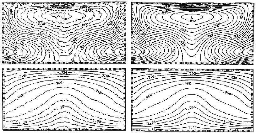
Figure: Comparison of Smoothed Particle Hydrodynamics with an Eulerian finite-difference calculation. The density (above) and temperature (below) contours for a stationary Rayleigh-Bénard flow are shown. Left: SPH; right: Euler. (From [Hoover 99], with kind permission by the author) vesely 2006
|