8.1.3 Smoothed Particle Hydrodynamics (SPH)

- PIC technique uses both Eulerian and Lagrangian elements. Average density within a cell = number of point particles in that cell.
- Can we represent the local fluid density without a grid?
Lucy [LUCY 77] and Gingold and Monaghan [GINGOLD 77,MONAGHAN 92]: load each particle with a spatially extended interpolation kernel $\Longrightarrow$Average local density = sum over the individual contributions.

Let $w(\mbox{$\bf r$}-\mbox{$\bf r_{i}$})$ denote the interpolation kernel centered around $\mbox{$\bf r_{i}$}$. Then the local density at $\mbox{$\bf r$}$ is

$$\langle \rho(\mbox{$\bf r$})\rangle = \sum_{i=1}^{N} m_{i}\, w(\mbox{$\bf r$}-\mbox{$\bf r_{i}$})$$ (8.33)

Generally, a property $A(\mbox{$\bf r$})$ is represented by its ``smoothed particle estimate''

$$\langle A(\mbox{$\bf r$})\rangle = \sum_{i=1}^{N} m_{i}\, \... ...(\mbox{$\bf r$}_{i})} \, w(\mbox{$\bf r$}-\mbox{$\bf r_{i}$})$$ (8.34)

Form of the interpolation kernel: Gaussian or polynomial
Example:

$$w(\mbox{$\bf s$}) = \frac{1}{\pi^{3/2}d^{3}} \, e^{- s^{2}/d^{2}}$$ (8.35)

with a width $d$ chosen such that the number of particles within $d$ is $N \approx 5$ in 2 dimensions and $N \approx 15$ for 3 dimensions.

Now rewrite the Lagrangian equations of motion 8.8, 8.9 and 8.11. in smoothed particle form.
Note: In the momentum equation $d \mbox{$\bf v$}/dt=- \nabla p / \rho$, interpolating $\rho$ and $\nabla p$ directly would not conserve linear and angular momentum [MONAGHAN 92].
$\Longrightarrow$Use the identity

$$\frac{1}{\rho}\, \nabla p = \nabla \left( \frac{p}{\rho}\right) + \frac{p}{\rho^{2}}\, \nabla \rho$$ (8.36)

and the SPH expressions for $A \equiv p/\rho$ and $A \equiv \rho$ to find

$$\frac{d \mbox{$\bf v$}_{i}}{dt} = - \sum_{k=1}^{N}m_{k} \le... ...2}} + \frac{p_{i}}{\rho_{i}^{2}} \right) \, \nabla_{i}w_{ik}$$ (8.37)

with $w_{ik} \equiv w(\mbox{$\bf r$}_{ik}) \equiv w(\mbox{$\bf r$}_{k}-\mbox{$\bf r$}_{i})$. If $w_{ik}$ is Gaussian, this equation describes the motion of particle $i$ under the influence of central pair forces

$$\mbox{$\bf F$}_{ik}=-m_{i}m_{k}\left( \frac{p_{k}}{\rho_{k}^... ...rho_{i}^{2}} \right) \frac{2 \mbox{$\bf r$}_{ik}}{d^{2}}w_{ik}$$ (8.38)

The SPH equivalents of the other Lagrangian flow equations are

$$\frac{d \rho_{i}}{dt} = \sum_{k=1}^{N}m_{k}\, \mbox{$\bf v$}_{ik} \cdot \nabla_{i}w_{ik}$$ (8.39)

where $\mbox{$\bf v$}_{ik} \equiv \mbox{$\bf v$}_{k}-\mbox{$\bf v$}_{i}$, and

$$\frac{d \epsilon_{i}}{dt} = - \sum_{k=1}^{N}m_{k}\, \left( \... ...i}^{2}} \right) \, \mbox{$\bf v$}_{ik} \cdot \nabla_{i}w_{ik}$$ (8.40)

Note: The density equation need not be integrated; just update all positions $\vec{r}_{i}$, then invoke equ. 8.33 to find $\rho(\mbox{$\bf r$}_{i})$. To update $\mbox{$\bf r$}_{i}$ the obvious relation

$$\frac{d \mbox{$\bf r$}_{i}}{dt} = \mbox{$\bf v$}_{i}$$ (8.41)

might be used; a better way is

$$\frac{d \mbox{$\bf r$}_{i}}{dt} = \mbox{$\bf v$}_{i} + \sum_... ...{N} \frac{m_{k}}{\bar{\rho}_{ik}} \mbox{$\bf v$}_{ik}\,w_{ik}$$ (8.42)

with $\bar{\rho}_{ik} \equiv (\rho_{i}+\rho_{k})/2$. This relation maintains angular and linear momentum conservation, with the additional advantage that nearby particles will have similar velocities [MONAGHAN 89].

To solve equs. 8.39, 8.37, 8.41 and 8.40, use any suitable algorithm (see Chapter 4). Popular schemes are the leapfrog algorithm, predictor-corrector and Runge-Kutta methods.

Example: Variant of the half-step technique ([MONAGHAN 89]):
Given all particle positions at time $t_{n}$, the local density at $\mbox{$\bf r$}_{i}$ is computed from 8.33. Writing equs. 8.37 and 8.40 as

$$\frac{d\mbox{$\bf v$}_{i}}{dt} = \mbox{$\bf F$}_{i} \;\;\;\; {\rm and} \;\;\; \frac{d\epsilon_{i}}{dt} = Q_{i}$$ (8.43)

compute the predictors

$$\mbox{$\bf v$}_{i}^{n+1}=\mbox{$\bf v$}_{i}^{n}+\Delta t \, ... ... \; \epsilon_{i}^{n+1}=\epsilon_{i}^{n}+\Delta t \, Q_{i}^{n}$$ (8.44)

and

$$\mbox{$\bf r$}_{i}^{n+1}=\mbox{$\bf r$}_{i}^{n}+\Delta t \, \mbox{$\bf v$}_{i}^{n}$$ (8.45)

Determine mid-point values of $\mbox{$\bf r$}_{i}$, $\mbox{$\bf v$}_{i}$ and $\epsilon_{i}$ according to

$$\mbox{$\bf r$}_{i}^{n+1/2} = \left( \mbox{$\bf r$}_{i}^{n}+\mbox{$\bf r$}_{i}^{n+1}\right) /2$$ (8.46)

etc. From these, compute mid-point values of $\rho_{i}$, $\mbox{$\bf F$}_{i}$ and $Q_{i}$ and insert these in correctors of the type

$$\mbox{$\bf v$}_{i}^{n+1}=\mbox{$\bf v$}_{i}^{n}+\Delta t \, \mbox{$\bf F$}_{i}^{n+1/2}$$ (8.47)

Here is an overview of the method:


Smoothed particle hydrodynamics (SPH)


Note: SPH is not restricted to compressible inviscid flow. Incompressibility may be introduced by using an equation of state that keeps compressibility below a few percent [MONAGHAN 92], and viscosity is added by an additional term in the equations of motions for momentum and energy, equs. 8.37 and 8.40:

$$\frac{d \mbox{$\bf v$}_{i}}{dt} = - \sum_{k=1}^{N} m_{k} \left( \frac{p_{k}}{\rho_{k}^{2}} + \frac{p_{i}}{\rho_{i}^{2}} + \Pi_{ik} \right) \, \nabla_{i}w_{ik}$$ (8.48)

$$\frac{d \epsilon_{i}}{dt} = - \sum_{k=1}^{N}m_{k}\, \left( \frac{p_{k}}{\rho_{k}^{2}} + \frac... ...{\rho_{i}^{2}} + \Pi_{ik} \right) \, \mbox{$\bf v$}_{ik} \cdot \nabla_{i}w_{ik}$$ (8.49)

The artificial viscosity term $\Pi_{ik}$ is modeled in the following way:

$$\Pi_{ik} = \left\{ \begin{array}{ll} \begin{array}{c} \unde... ..._{ik} \cdot \mbox{$\bf r$}_{ik} \geq 0$} \end{array} \right.$$ (8.50)

where $c$ is the speed of sound, $\mu$ is defined by

$$\mu_{ik} \equiv \frac{ ( \mbox{$\bf v$}_{ik} \cdot \mbox{$\bf r$}_{ik}) \, d}{r_{ik}^{2}+ \eta^{2}}$$ (8.51)

and $c_{ik} \equiv c_{k}- c_{i}$ and $\bar{c}_{ik} \equiv (c_{i}+c_{k})/2$ etc.
This form of $\Pi$ introduces the effects of shear and bulk viscosity. The parameters $\alpha$ and $\beta$ should be near $\alpha = 1$ and $\beta = 2$ for best results [MONAGHAN 92]. The quantity $\eta$ prevents singularities for $r_{ik} \approx 0$. It should be chosen such that $\eta^{2}=0.01 d^{2}$.

Additional features:
Thermal conduction may be included. See [MONAGHAN 89].
Interfaces: Introduce dummy particles on the far side of the boundary. By picking the properties of these particles appropriately one can mimick a free surface or a ``sticky'' solid boundary. See Nugent and Posch [NUGENT 00] for free surfaces, and Ivanov [IVANOV 00] for rough interfaces

Sample application: ``Rayleigh-Bénard'' convection
A fluid layer is heated carefully from below and cooled from above. $\Longrightarrow$Formation of stable convective rolls transporting heat from the bottom to the top. See the Figure for a match between SPH and an Euler-type calculation [HOOVER 99]:
- Computing times comparable for both calculations
- Results are in good agreement
- Fluctuations in SPH (like in any particle-type calculation), none in Euler
- SPH code is quite simple - similar to an MD program; Euler code very massive


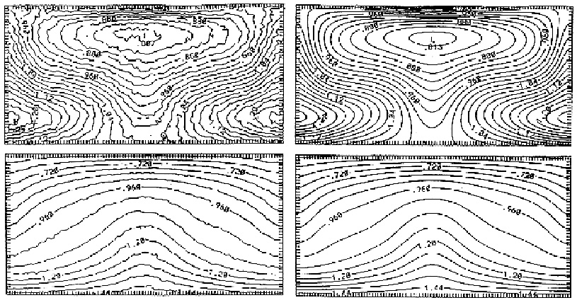
Comparison of Smoothed Particle Hydrodynamics with an Eulerian finite-difference calculation. The density (above) and temperature (below) contours for a stationary Rayleigh-Bénard flow are shown. Left: SPH; right: Euler. (From [HOOVER 99], with kind permission by the author)