| |
|
< BACK TO INDEX
|
HSCM News
Mar 2008
|
Go to:
> LJ Lines / Tetrachoric series
> Bare Cylinders again
> NPT-MC Snapshot
-
LJ Lines / Tetrachoric series
[This is mainly for Kike:]
In my fortran codes ljsticks.f and ljs_rc.f (and similar) I have to
compute the bivariate normal cumulative distribution bvnc depending
on a pair of coordinates $(x,y)$ in $[-\infty,\infty]$ and a
correlation $\rho$ in $[-1,1]$. When $\rho^{2} \rm{<} 0.5$ the
distribution is best represented by the tetrachoric series,
otherwise we use Vasicek's complementary algorithm.
Now, the tetra series has some stability problems when we go to
a larger number of terms. I have therefore derived a more stable
series which may be switched on in my code. Here are the details.
Let us call the bivariate distribution (bvnc in the code)
$ N_{2}(x,y,\rho)$. The tetra series (Abramovitz etc.) is
$
N_{2}(x,y,\rho) =
N(x)\, N(y) +n(x)\, n(y)
\sum \limits_{k=0}^{m} \frac{\textstyle 1}{(\textstyle k+1)!}
He_{k}(x) \, He_{k}(y) \, \rho^{k+1}
$
where $n(x)$ is the 1 D normal density with cumulative distribution
$N(x)$, and $He_{k}$ are the "probabilists'
Hermite polynomials" defined by
$He_{k+1}(x)=x He_{k}(x)-k He_{k-1}(x)$;
$He_{0}(x)=1$; $He_{1}(x)=x$.
It is tempting now to use this recursive definition of the Hermite
polynomials, but they tend to attain large numerical values - as
does the denominator $1 / (k+1)!$. To avoid quotients of large numbers
we may define the auxiliary terms
$
f_{k} \equiv
\frac{\textstyle He_{k}(x) \, He_{k}(y) }{ \textstyle (k+1)!},
\;\;\;\;\;\;
g_{k} \equiv
\frac{\textstyle He_{k-1}(x) \, He_{k}(y) }{ \textstyle (k+1)!},
\;\;\;\;\;\;
h_{k} \equiv
\frac{\textstyle He_{k-1}(x) \, He_{k}(y) }{\textstyle (k+1)!}
$
which obey the recursion relations
$
\begin{eqnarray}
f_{k} &=&
\frac{\textstyle xy }{ \textstyle (k+1)} f_{k-1}+
\frac{\textstyle (k-1)^{2} }{ \textstyle k(k+1)} f_{k-2}-
\frac{\textstyle (k-1)x }{ \textstyle (k+1)} g_{k-1}-
\frac{\textstyle (k-1)y }{ \textstyle (k+1)} h_{k-1}
\\
g_{k} &=&
\frac{\textstyle x }{ \textstyle (k+1)} f_{k-1}-
\frac{\textstyle (k-1) }{ \textstyle (k+1)} h_{k-1}
\\
h_{k} &=&
\frac{\textstyle y }{ \textstyle (k+1)} f_{k-1}-
\frac{\textstyle (k-1) }{ \textstyle (k+1)} g_{k-1}
\end{eqnarray}
$
|
-
Bare Cylinders again
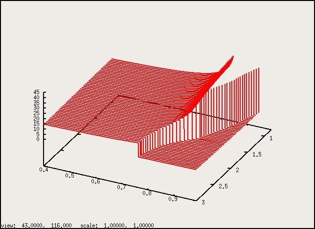
I have now done a complete sweep with $l_{1}=10.$, $l_{2}=0.8-7.0$, $d_{1}=d_{2}=1$
and concentration $X_{2}=0.1-0.99$. Again, the search strategy was simply to
increase $\eta$ and $k$ until $ |S(\eta,k)|$ crossed zero.
Starting at this point the nearest minimum of $S(\eta,k)$ with $S=0$ was
found using a 2D Newton-Raphson strategy.
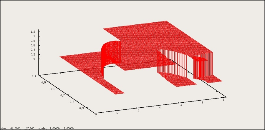
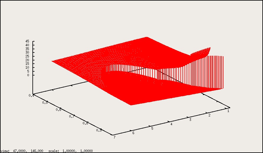
The graphs look much the same as before. I left off the low $X_{2}$ part as it is
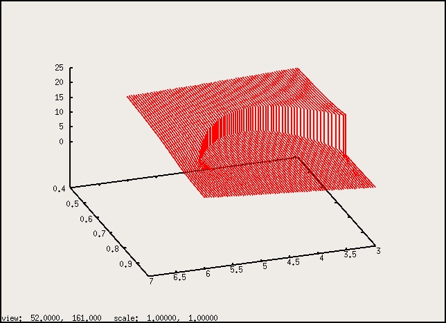
really flat. The steps in $\lambda$, looking like the teeth of a whale, are
just an indication of zero smectic wave number.
All the data displayed here may be downloaded from this directory; they are
packed as the file "Bbcmar08.tar.gz". [Kike: these are the files you already
have, except that now all $\lambda$ are positive, even if $k \approx 0$ is
numerically negative...]. There are also some useful gnuplot scripts.
|
Figure 1: Phase surface, total, for BC mixtures.
|
| |
|
Figure 2: Smectic wave length $\lambda(l_{2},X_{2})$ for BC mixtures.
|
|
|
|
Figure 3: Detail in phase surface.
|
|
Figure 4: Detail in the $\lambda$ surface.
|
I have not yet included the results pertaining to the left part in Van Roij's
Figure 3d,
for $l_{1}=10$ and $l_{2}=1$, and $X_{2} \rm{>} 0.89$ (in our
notation; they have $x \rm{<} 0.11$). Anyway, here are some
results. In that region I get two
branches of states with $|S|=0$ and $dS/dk=0$, at low and high packing
densities. Here I show you first the table, then the graph. In the table,
"T T" means "smectic=true / demix=true" etc. Thus, "T T" denotes a
smectically demixed state, "T F" a smectic but mixed state.
| Low $\eta$ branch: |
| $X_{2}$ | $\eta$ |
$k$ | |
| 0.8600 | 0.3504436e0 | 0.1690574e0 | T T |
| 0.8700 | 0.3471773e0 | 0.1428434e0 | T T |
| 0.8800 | 0.3440657e0 | 0.1069540e0 | T T |
| 0.8850 | 0.3425854e0 | 0.8133598e-1 | T T |
| 0.8880 | 0.3417263e0 | 0.5999829e-1 | T T |
| 0.8890 | 0.3414453e0 | 0.5072583e-1 | T T |
| 0.8900 | 0.3411672e0 | 0.3918362e-1 | T T |
| 0.8910 | 0.3408919e0 | 0.2205258e-1 | T T |
| 0.8911 | 0.3408645e0 | 0.1951366e-1 | T T |
| 0.8912 | 0.3408372e0 | 0.1658717e-1 | T T |
| 0.8913 | 0.3408099e0 | 0.1301422e-1 | T T |
| 0.8914 | 0.3407826e0 | 0.0796805e-1 | T T |
| *** here k --> 0! |
| 0.8915 | 0.3407554e0 | 0.1d-7 | F T |
| 0.8920 | 0.3406210e0 | 0.1d-7 | F T |
| 0.8930 | 0.3403615e0 | 0.1d-7 | F T |
| High $\eta$ branch: |
| $X_{2}$ | $\eta$ |
$k$ | |
| 0.888 | 1.1583904e0 | 0.4289670e1 | T F |
| 0.889 | 1.1533599e0 | 0.4289944e1 | T F |
| 0.890 | 1.1483279e0 | 0.4290221e1 | T F |
| 0.895 | 1.1231434e0 | 0.4291666e1 | T F |
| 0.900 | 1.0979175e0 | 0.4293220e1 | T F |
| 0.910 | 1.0473359e0 | 0.4296722e1 | T F |
| 0.920 | 0.9965697e0 | 0.4300891e1 | T F |
| 0.930 | 0.9456009e0 | 0.4305976e1 | T F |
| 0.940 | 0.8944036e0 | 0.4312373e1 | T F |
| 0.950 | 0.8429376e0 | 0.4320750e1 | T F |
| 0.960 | 0.7911352e0 | 0.4332333e1 | T F |
| 0.970 | 0.7388689e0 | 0.4349635e1 | T F |
| 0.980 | 0.6858665e0 | 0.4378557e1 | T F |
| 0.990 | 0.6315195e0 | 0.4431985e1 | T F |
| 0.995 | 0.6036269e0 | 0.4466310e1 | T F |
| 0.998 | 0.5867204e0 | 0.4483845e1 | T F |
| 0.999 | 0.5810705e0 | 0.4488838e1 | T F |
|
|
|
|
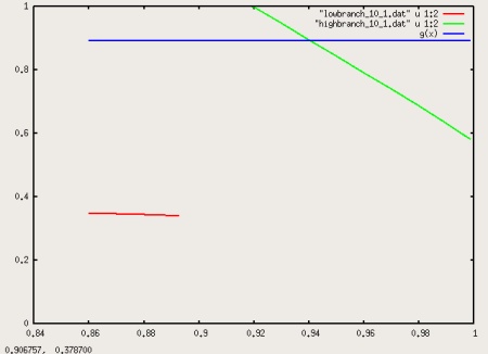
Figure 5: Packing density at bifurcation, for the 10:1
system. Compare to Van Roij-Mulder, Fig. 3d.
|
|
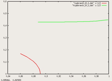
Figure 6: Wave number at bifurcation.
|
Figure 5 is roughly the mirror image of Van Roij-Mulder's Fig. 3d,
except that I have included the blue line to denote the
maximum attainable packing density ($0.89$ for very long
hex packed cylinders.) The low-density branch ends exactly
at $X_{2}=0.8915$, where the smectic wave length diverges
(see Fig. 6). At this $X_{2}$ we can also find a high-density branch
with smectic (S1) structure, but this branch starts out far beyond
the physically meaningful $\eta$. Only for $X_{2}$ larger than
about $0.94$ the packing density falls below the limit of $0.89$.
|
-
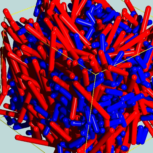
NPT-MC Snapshot
|
Figure 7: N=864 hard SC particles; NPT MC at
$X_{2}=0.6$; $p=0.6$; $\eta=0.33$; $P_{2}=0.49$; not quite
equilibrated.
|
Next run will be for N=1372 and $X_{2}=0.4$, as agreed with Luis and Kike.
^ UP TO TOP
< BACK TO INDEX
|
vesely mar-2008
|