| Franz J. Vesely > CompPhys Tutorial > Partial Differential Equations |
5.1 Initial Value Problems I: Conservative-hyperbolic DE
$
\frac{\textstyle \partial u}{\textstyle \partial t} =
- \frac{\textstyle \partial j}{\textstyle \partial x}
$
Best (i.e. most stable, exact, etc.): Lax-Wendroff technique Approach to Lax-Wendroff via: FTCS $\Longrightarrow$ Lax $\Longrightarrow$ Leapfrog Subsections
5.1.1 FTCS Scheme; Stability AnalysisWriting $u_{j}^{n} \equiv u(x_{j},t_{n})$ and using DNGF for the time derivative (FT, "forward-time"), and DST for the space derivative (CS, for "centered-space"), we write $\partial u/\partial t = - \partial j/\partial x$ as
$
\begin{eqnarray}
\frac{\textstyle 1}{\textstyle \Delta t} \left[ u_{j}^{n+1}- u_{j}^{n} \right]
& \approx &
- \frac{\textstyle 1}{\textstyle 2 \Delta x}
\left[ j_{j+1}^{n}- j_{j-1}^{n} \right]
\end{eqnarray}
$
$
\begin{eqnarray}
&&
u_{j}^{n+1}= u_{j}^{n}-\frac{\textstyle \Delta t}{\textstyle 2 \Delta x}
\left[ j_{j+1}^{n}- j_{j-1}^{n} \right]
\end{eqnarray}
$
This may be symbolized as follows: 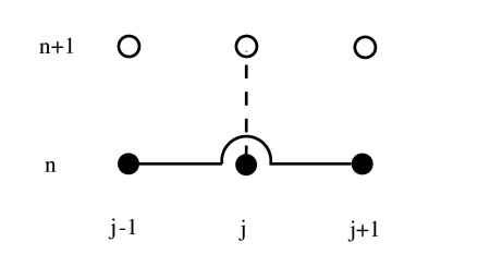
Stability analysis (J. v. Neumann): At time $t_{n}$, expand $u(x,t)$:
$
\begin{eqnarray}
u_{j}^{n}&=& \sum_{k} U_{k}^{n} e^{\textstyle ikx_{j}}
\end{eqnarray}
$
where $ k=2\pi l/L \;\; (l=0,1,\dots)$. Insert this in $u_{j}^{n+1}=T[u_{j'}^{n}]$ to find each Fourier component's propagation law, $U_{k}^{n+1}=g(k) U_{k}^{n}$. $\Longrightarrow$ Stable if $| g(k) | \leq 1 \;\;{\rm for \; all \; k}$. Application to FTCS + advective equation with $j=cu$:
$
\begin{eqnarray}
g(k) \, U_{k}^{n} e^{\textstyle ikj \Delta x} &=&
U_{k}^{n} \, e^{\textstyle ikj \Delta x}
- \frac{\textstyle c \Delta t}{\textstyle 2 \Delta x} U_{k}^{n}
[e^{\textstyle ik(j+1)\Delta x} - e^{\textstyle ik(j-1)\Delta x}]
\end{eqnarray}
$
or
$
\begin{eqnarray}
g(k) & = & 1- \frac{\textstyle ic \Delta t}{\textstyle \Delta x} \sin k \Delta x
\end{eqnarray}
$
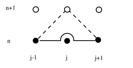
Obviously, $\vert g(k)\vert > 1$ for any $k$; the FTCS method is inherently unstable. 5.1.2 Lax SchemeReplacing in the FTCS formula the term $u_{j}^{n}$ by its spatial average $[u_{j+1}^{n}+ u_{j-1}^{n}]/2$, we approximate $\partial u/\partial t = - \partial j/\partial x$ by
$
\begin{eqnarray}
&&
u_{j}^{n+1} = \frac{1}{2}
\left[ u_{j+1}^{n}+ u_{j-1}^{n} \right]
-\frac{\textstyle \Delta t}{\textstyle 2 \Delta x}
\left[ j_{j+1}^{n}- j_{j-1}^{n} \right]
\end{eqnarray}
$
Insert Fourier expanded $u(x)$ in Lax formula to find
$
\begin{eqnarray}
g(k)= \cos k \Delta x -i \frac{\textstyle c \Delta t}{\textstyle \Delta x}
\sin k \Delta x
\end{eqnarray}
$
The condition $\vert g(k)\vert \leq 1$ is tantamount to
$
\begin{eqnarray}
&&
\frac{\textstyle |c| \Delta t}{\textstyle \Delta x} \leq 1
\end{eqnarray}
$
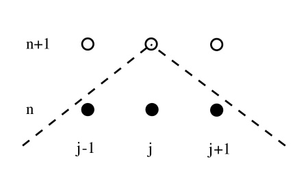
Region below the dashed line: physically relevant for $u_{j}^{n+1}$, according to $x(t_{n+1})=x(t_{n})\pm |c| \Delta t$ Close scrutiny shows that LAX solves not the original PDE but
$
\begin{eqnarray}
\frac{\textstyle \partial u}{\textstyle \partial t} & = &
-c \frac{\textstyle \partial u}{\textstyle \partial x}
+ \frac{\textstyle (\Delta x)^{2}}{\textstyle 2 \Delta t}
\frac{\textstyle \partial^{2} u}{\textstyle \partial x^{2}}
\end{eqnarray}
$
The additional diffusive term makes the method stable. However, it is an artefact and should be small:
$
\begin{eqnarray}
|c| \Delta t & >> & \frac{\textstyle \Delta x}{\textstyle 2}
\frac{\textstyle |\delta^{2} u|}{\textstyle |\delta u|}
\end{eqnarray}
$
5.1.3 Leapfrog Scheme (LF)Use DST for $\partial/\partial t$: $ \partial u /\partial t \approx (u^{n+1}-u^{n-1})/2\Delta t$ to find the leapfrog expression
$
\begin{eqnarray}
&&
u_{j}^{n+1}- u_{j}^{n-1}=
-\frac{\textstyle \Delta t}{\textstyle \Delta x}
\left[ j_{j+1}^{n}- j_{j-1}^{n} \right]
\end{eqnarray}
$
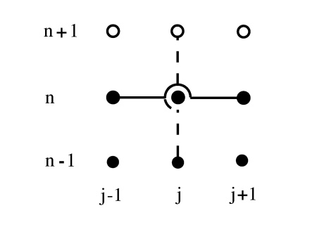
Stability requires once more that $c\Delta t/\Delta x \leq 1$ (CFL condition) 5.1.4 Lax-Wendroff Scheme (LW)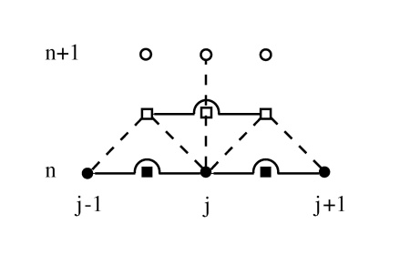
Stability: Once more assuming $j=cu$ and using the ansatz $U_{k}^{n+1}= g(k) U_{k}^{n}$ we find
$
\begin{eqnarray}
g(k)&=&1-ia \sin k \Delta x -a^{2}(1-\cos k \Delta x),
\end{eqnarray}
$
with $a=c \Delta t/ \Delta x$. The requirement $\vert g\vert^{2}\leq 1$ leads once again to the CFL condition, $c\Delta t/\Delta x \leq 1$. 5.1.5 Lax and Lax-Wendroff in Two Dimensions
$
\frac{\textstyle \partial u}{\textstyle \partial t} =
-\frac{\textstyle \partial j_{x}}{\textstyle \partial x}
-\frac{\textstyle \partial j_{y}}{\textstyle \partial y}
$
(advective case: $j_{x}=c_{x}u$ and $j_{y}=c_{y}u$) Lax scheme:
$
u_{i,j}^{n+1} = \frac{1}{4}
\left[ u_{i+1,\,j}^{n}+u_{i,j+1}^{n}+u_{i-1,j}^{n}+u_{i,j-1}^{n}\right]
-\frac{\textstyle \Delta t}{\textstyle 2 \Delta x}
\left[ j_{x,i+1,j}^{n}-j_{x,i-1,j}^{n}\right]
- \frac{\textstyle \Delta t}{\textstyle 2 \Delta y}
\left[j_{y,i,j+1}^{n}-j_{y,i,j-1}^{n}\right]
$
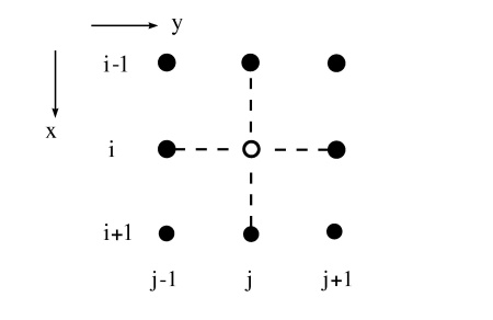
Figure: Lax method in two dimensions Lax-Wendroff: For the second stage (half-step leapfrog) we need $j_{x,i+1/2,j-1/2}^{n+1/2}$ etc., which requires $u_{i+1/2,j-1/2}^{n+1/2}$, which must be determined from $u_{i,j-1/2}^{n},$ $u_{i+1,j-1/2}^{n}$ etc. But: quantities with half-step spatial indices ($\scriptstyle i+1/2$, $\scriptstyle j-1/2$ etc.) are given at half-step times ($t_{n+1/2}$) only. Modifying the LW scheme to allow for this, we have Lax-Wendroff in 2 dimensions:
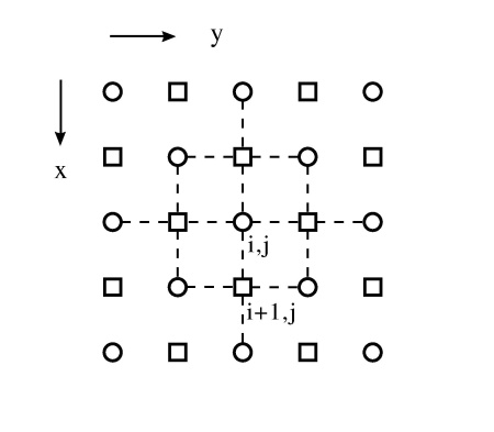
Figure: First stage (= Lax) in the 2-dimensional LW method: $ \textstyle \circ $ ... $t_{n},t_{n+1}$,  ... $t_{n+1/2}$ ... $t_{n+1/2}$
For $u_{i,j}^{n+1}$ only the points $\textstyle \circ $ (at $t_{n}$) are used; for $u_{i+1,j}^{n+1}$ we use the points .
Problem: Drift between subgrids $\textstyle \circ $ and .
Solution: If the given PDE contains a diffusive term, this guarantees coupling. Otherwise, artificially add a small diffusive term. Stability analysis: Fourier modes are now 2-dimensional:
$u(x,y)=\sum_{k} \sum_{l} U_{k,l} e^{\textstyle ikx+ily}$
Assuming $\Delta x = \Delta y$ we find the CFL condition
$
\Delta t \leq \frac{\textstyle \Delta x}{\textstyle \sqrt{2}
\sqrt{c_{x}^{2}+c_{y}^{2}}}
$
5.1.6 Resumé: Conservative-hyperbolic DE
$
\begin{eqnarray}
\frac{\textstyle \partial u}{\textstyle \partial t} & = &
- \frac{\textstyle \partial j}{\textstyle \partial x}
\end{eqnarray}
$
- Use Lax-Wendroff! - If not, use at least Lax, but see that in addition to CFL
$
\begin{eqnarray}
|c| \Delta t &>>& \frac{\textstyle \Delta x}{\textstyle 2}
\frac{\textstyle |\delta^{2} u|}{\textstyle |\delta u|}
\end{eqnarray}
$
- Forget FTCS and Leapfrog! To test the various methods, let us apply them to the 1D wave equation. When altering the propagation velocity $c$, the time step $\Delta t$, or the grid width $\Delta x$, keep in mind the operation regions of the different algorithms: FTCS - unstable LAX, LEAPFROG, LAX-WENDROFF - CFL condition $|c| \Delta t / \Delta x \leq 1$
vesely 2005-10-10
|
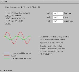 Applet Hpde1: