Home     Back to book

Franz J. Vesely: Computational Physics - An Introduction Second Edition Kluwer Academic / Plenum Publishers, New York-London 2001. ISBN 0-306-46631-7

Here are a few errata I have detected since publication

Es irrt der Mensch, solang er strebt  [Goethe] If anything can go wrong, it will  [Murphy]

Status: Sep-04

Page 34: Equation 2.53 should read

$$a_{ii} x_{i}^{(k+1)} = b_{i} - \sum_{j > i} a_{ij} x_{j}^{(k)} - \sum_{j<i} a_{ij} x_{j}^{(k+1)} \; ; \;\;\; i=1,\dots,N$$

[May 02; thanks to Steve Knudsen] Page 34: Equation 2.58 should read

$$\left[ \mbox{${\bf D}$} + \mbox{${\bf L}$} \right] \cdot \mbox{$\bf x$}_{k+1} = \omega \mbox{$\bf b$} - \left[ \omega \mbox{${\bf R}$} - (1-\omega) \mbox{${\bf A}$} \right] \cdot \mbox{$\bf x$}_{k}$$

[and in 2.59, the last $(k)$ should be a superscipt]

[May 02; thanks to Steve Knudsen] Page 39: Equation 2.72 should read

$$\vec{h}_{1}= \vec{g}_{1}-\frac{(\mbox{${\bf A}$} \cdot \vec... ... \mbox{${\bf A}$} \cdot \vec{g}_{0} \right\vert^{2}} \nonumber$$

(Note that $\vec{h}_{0} \equiv \vec{g}_{0}$). Accordingly, eq. 2.75 should be

$$\vec{h}_{2} = \vec{g}_{2} - \frac{(\mbox{${\bf A}$} \cdot \... ... \mbox{${\bf A}$} \cdot \vec{h}_{1} \right\vert^{2}} \nonumber$$

With these corrections the example calculation following eq. 2.77 converges faster - as it should.

[Sep 04; thanks to Greg Hammett] Page 82: The last five lines should read:

In our simple example the fitness is bound to the value $f_{i} \equiv f(x_{i}^{0})$: the lower $f_{i}$, the higher the fitness of $x_{i}^{0}$. It is always possible, and convenient, to assign the fitness $g_{i} \equiv g(x_{i}^{0})$ such that it is positive definite.

A relative fitness, or probability of reproduction, is defined as $p_{i} \equiv g_{i}/\sum_{i=1}^{N}g_{i}$. It has all the markings of a probability density, and accordingly we may also ...

[Dec 03]

Page 117: Equ. 4.153 should read:

$$\mbox{$\bf q$}_{n+1}=\mbox{$\bf q$}_{n}+\mbox{$\bf P$}(\mbox... ...mbox{$\bf p$}_{n}+\mbox{$\bf F$}(\mbox{$\bf q$}_{n+1})\Delta t$$

- Somewhat later, the sentence beginning ``Incidentally, ..'' should read:

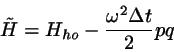
A very similar first-order symplectic scheme, also known as the Euler-Cromer algorithm,

$$\mbox{$\bf p$}_{n+1}=\mbox{$\bf p$}_{n}+\mbox{$\bf F$}(\mbox... ...mbox{$\bf q$}_{n}+\mbox{$\bf P$}(\mbox{$\bf p$}_{n+1})\Delta t$$

exactly conserves the perturbed Hamiltonian

$$\tilde{H}=H_{ho}-\frac{\textstyle \omega^{2} \Delta t}{\textstyle 2}pq$$

When applied to oscillator-like equations of motion it is a definite improvement over the (unstable) Euler-Cauchy method ...

[Dec 03, thanks to Denis Donnelly] Page 154: Equ. 5.137 is printed as

$$\beta_{l}= 2 \cos\left[ \frac{2(l-1)\pi}{2^{p+1}}\right]$$

but should read

$$\beta_{l}= 2 \cos\left[ \frac{(2l-1)\pi}{2^{p+1}}\right]$$

Note: the same error appears in Hockney's book

[Jan 04, thanks to the class of 03/04] Page 168: The text following equ. 6.8 should read

... where $u^{*} \equiv u_{LJ}/\epsilon$ and ...

[Oct 03] Page 187: Eq. 6.60: the second term in the brackets should read

$$\sum_{\vec{n}} \frac{L^{3}}{\vert\vec{r}_{i,j,\vec{n}}\vert}F(\eta \vert\vec{r}_{i,j,\vec{n}}\vert)$$ (1)

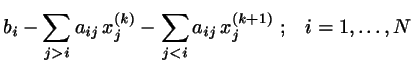
[Apr 06] Page 217: Eq. 8.12: should be

$$\frac{d e}{dt} = - (e+p) \nabla \cdot \mbox{$\bf v$} -(\mbox{$\bf v$} \cdot \nabla)\, p$$

$$= -e (\nabla \cdot \mbox{$\bf v$}) - \nabla \cdot (p \mbox{$\bf v$})$$ (2)

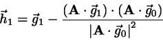
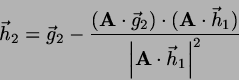
[May 06] Page 218: Eq. 8.18: first line should be

$$e_{j}^{n+1} = \frac{1}{2}\left(e_{j+1}^{n}+e_{j-1}^{n} \right)$$ (3)

$$- \dots$$ (4)

[May 06] Page 232: In Figure 8.6 the shading of some cells is barely visible.



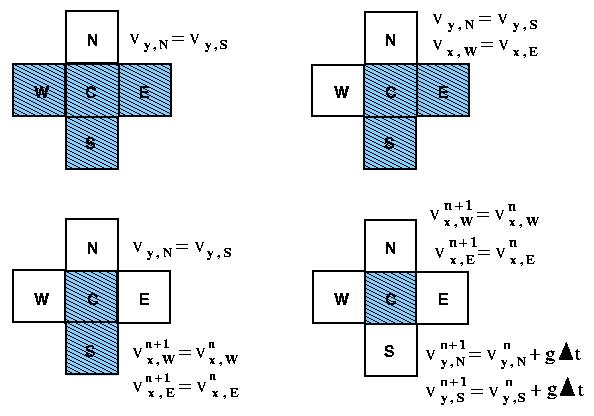
MAC method: the 4 types of surface cells and the appropriate boundary conditions for $v_{x}, v_{y}$ (see POTTER).

[May 02]